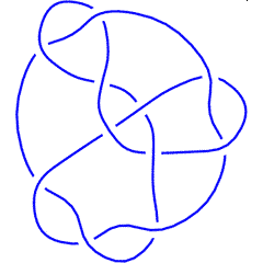
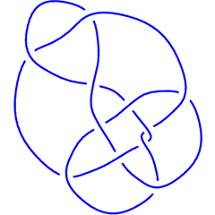
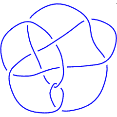
K11n129

K11n128

K11n130

(Knotscape image)	See the full Hoste-Thistlethwaite Table of 11 Crossing Knots. Visit K11n129 at Knotilus!

Knot presentations

Planar diagram presentation	X4251 X10,3,11,4 X5,19,6,18 X7,14,8,15 X9,16,10,17 X2,11,3,12 X13,20,14,21 X15,8,16,9 X17,1,18,22 X19,12,20,13 X21,7,22,6
Gauss code	1, -6, 2, -1, -3, 11, -4, 8, -5, -2, 6, 10, -7, 4, -8, 5, -9, 3, -10, 7, -11, 9
Dowker-Thistlethwaite code	4 10 -18 -14 -16 2 -20 -8 -22 -12 -6

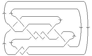
A Braid Representative
A Morse Link Presentation

Three dimensional invariants

Symmetry type Chiral Unknotting number $\{1,2\}$ 3-genus 3 Bridge index 3 Super bridge index Missing Nakanishi index Missing Maximal Thurston-Bennequin number Data:K11n129/ThurstonBennequinNumber Hyperbolic Volume 11.7204 A-Polynomial See Data:K11n129/A-polynomial

[edit Notes for K11n129's three dimensional invariants]

Four dimensional invariants

Smooth 4 genus Missing Topological 4 genus Missing Concordance genus $3$ Rasmussen s-Invariant 2

[edit Notes for K11n129's four dimensional invariants]

Polynomial invariants

Alexander polynomial	$t^3-4 t^2+10 t-13+10 t^{-1} -4 t^{-2} + t^{-3}$
Conway polynomial	$z^6+2 z^4+3 z^2+1$
2nd Alexander ideal (db, data sources)	$\{1\}$
Determinant and Signature	{ 43, -2 }
Jones polynomial	$q-3+5 q^{-1} -6 q^{-2} +8 q^{-3} -7 q^{-4} +6 q^{-5} -4 q^{-6} +2 q^{-7} - q^{-8}$
HOMFLY-PT polynomial (db, data sources)	$-z^4 a^6-3 z^2 a^6-3 a^6+z^6 a^4+5 z^4 a^4+10 z^2 a^4+6 a^4-2 z^4 a^2-5 z^2 a^2-3 a^2+z^2+1$
Kauffman polynomial (db, data sources)	$z^5 a^9-3 z^3 a^9+z a^9+2 z^6 a^8-5 z^4 a^8+z^2 a^8+3 z^7 a^7-9 z^5 a^7+8 z^3 a^7-3 z a^7+3 z^8 a^6-11 z^6 a^6+17 z^4 a^6-11 z^2 a^6+3 a^6+z^9 a^5-7 z^5 a^5+15 z^3 a^5-6 z a^5+4 z^8 a^4-16 z^6 a^4+30 z^4 a^4-21 z^2 a^4+6 a^4+z^9 a^3-3 z^7 a^3+6 z^5 a^3-z^3 a^3-2 z a^3+z^8 a^2-3 z^6 a^2+9 z^4 a^2-11 z^2 a^2+3 a^2+3 z^5 a-5 z^3 a+z^4-2 z^2+1$
The A2 invariant	$-q^{24}-2 q^{20}-q^{18}+2 q^{16}+3 q^{12}+q^{10}+q^8+q^6-2 q^4+q^2-1+ q^{-4}$
The G2 invariant	Data:K11n129/QuantumInvariant/G2/1,0

Further Quantum Invariants

K11n129 Quantum Invariants.

Computer Talk

The above data is available with the Mathematica package KnotTheory`, as shown in the (simulated) Mathematica session below. Your input (in red) is realistic; all else should have the same content as in a real mathematica session, but with different formatting. This Mathematica session is also available (albeit only for the knot 5_2) as the notebook PolynomialInvariantsSession.nb.

(The path below may be different on your system, and possibly also the KnotTheory` date)

In[1]:=

AppendTo[$Path, "C:/drorbn/projects/KAtlas/"]; << KnotTheory`

Loading KnotTheory` version of August 31, 2006, 11:25:27.5625. Read more at http://katlas.math.toronto.edu/wiki/KnotTheory.

In[3]:=

K = Knot["K11n129"];

In[4]:=

Alexander[K][t]

KnotTheory::loading: Loading precomputed data in PD4Knots`.

Out[4]=

$t^3-4 t^2+10 t-13+10 t^{-1} -4 t^{-2} + t^{-3}$

In[5]:=

Conway[K][z]

Out[5]=

$z^6+2 z^4+3 z^2+1$

In[6]:=

Alexander[K, 2][t]

KnotTheory::credits: The program Alexander[K, r] to compute Alexander ideals was written by Jana Archibald at the University of Toronto in the summer of 2005.

Out[6]=

$\{1\}$

In[7]:=

{KnotDet[K], KnotSignature[K]}

Out[7]=

{ 43, -2 }

In[8]:=

Jones[K][q]

KnotTheory::loading: Loading precomputed data in Jones4Knots`.

Out[8]=

$q-3+5 q^{-1} -6 q^{-2} +8 q^{-3} -7 q^{-4} +6 q^{-5} -4 q^{-6} +2 q^{-7} - q^{-8}$

In[9]:=

HOMFLYPT[K][a, z]

KnotTheory::credits: The HOMFLYPT program was written by Scott Morrison.

Out[9]=

$-z^4 a^6-3 z^2 a^6-3 a^6+z^6 a^4+5 z^4 a^4+10 z^2 a^4+6 a^4-2 z^4 a^2-5 z^2 a^2-3 a^2+z^2+1$

In[10]:=

Kauffman[K][a, z]

KnotTheory::loading: Loading precomputed data in Kauffman4Knots`.

Out[10]=

$z^5 a^9-3 z^3 a^9+z a^9+2 z^6 a^8-5 z^4 a^8+z^2 a^8+3 z^7 a^7-9 z^5 a^7+8 z^3 a^7-3 z a^7+3 z^8 a^6-11 z^6 a^6+17 z^4 a^6-11 z^2 a^6+3 a^6+z^9 a^5-7 z^5 a^5+15 z^3 a^5-6 z a^5+4 z^8 a^4-16 z^6 a^4+30 z^4 a^4-21 z^2 a^4+6 a^4+z^9 a^3-3 z^7 a^3+6 z^5 a^3-z^3 a^3-2 z a^3+z^8 a^2-3 z^6 a^2+9 z^4 a^2-11 z^2 a^2+3 a^2+3 z^5 a-5 z^3 a+z^4-2 z^2+1$

"Similar" Knots (within the Atlas)

Same Alexander/Conway Polynomial: {10_151, K11n54,}

Same Jones Polynomial (up to mirroring, $q\leftrightarrow q^{-1}$): {9_21,}

Computer Talk

The above data is available with the Mathematica package KnotTheory`. Your input (in red) is realistic; all else should have the same content as in a real mathematica session, but with different formatting.

(The path below may be different on your system, and possibly also the KnotTheory` date)

In[1]:=

AppendTo[$Path, "C:/drorbn/projects/KAtlas/"]; << KnotTheory`

Loading KnotTheory` version of May 31, 2006, 14:15:20.091. Read more at http://katlas.math.toronto.edu/wiki/KnotTheory.

In[3]:=

K = Knot["K11n129"];

In[4]:=

{A = Alexander[K][t], J = Jones[K][q]}

KnotTheory::loading: Loading precomputed data in PD4Knots`.

KnotTheory::loading: Loading precomputed data in Jones4Knots`.

Out[4]=

{ $t^3-4 t^2+10 t-13+10 t^{-1} -4 t^{-2} + t^{-3}$, $q-3+5 q^{-1} -6 q^{-2} +8 q^{-3} -7 q^{-4} +6 q^{-5} -4 q^{-6} +2 q^{-7} - q^{-8}$ }

In[5]:=

DeleteCases[Select[AllKnots[], (A === Alexander[#][t]) &], K]

KnotTheory::loading: Loading precomputed data in DTCode4KnotsTo11`.

KnotTheory::credits: The GaussCode to PD conversion was written by Siddarth Sankaran at the University of Toronto in the summer of 2005.

Out[5]=

{10_151, K11n54,}

In[6]:=

DeleteCases[ Select[ AllKnots[], (J === Jones[#][q] || (J /. q -> 1/q) === Jones[#][q]) & ], K ]

KnotTheory::loading: Loading precomputed data in Jones4Knots11`.

Out[6]=

{9_21,}

Vassiliev invariants

V2 and V3:

(3, -6)

V2,1 through V6,9:

V2,1 V3,1 V4,1 V4,2 V4,3 V5,1 V5,2 V5,3 V5,4 V6,1 V6,2 V6,3 V6,4 V6,5 V6,6 V6,7 V6,8 V6,9 $12$ $-48$ $72$ $190$ $18$ $-576$ $-1024$ $-96$ $-208$ $288$ $1152$ $2280$ $216$ $\frac{52271}{10}$ $-\frac{3946}{15}$ $\frac{33742}{15}$ $\frac{913}{6}$ $\frac{2671}{10}$

V_2,1 through V_6,9 were provided by Petr Dunin-Barkowski <barkovs@itep.ru>, Andrey Smirnov <asmirnov@itep.ru>, and Alexei Sleptsov <sleptsov@itep.ru> and uploaded on October 2010 by User:Drorbn. Note that they are normalized differently than V₂ and V₃.

Khovanov Homology

The coefficients of the monomials $t^rq^j$ are shown, along with their alternating sums $\chi$ (fixed $j$, alternation over $r$). The squares with yellow highlighting are those on the "critical diagonals", where $j-2r=s+1$ or $j-2r=s-1$, where $s=$-2 is the signature of K11n129. Nonzero entries off the critical diagonals (if any exist) are highlighted in red.

\   r    \    j   \ -7 -6 -5 -4 -3 -2 -1 0 1 2 χ 3                   1 1 1                 2   -2 -1               3 1   2 -3             4 3     -1 -5           4 2       2 -7         3 4         1 -9       3 4           -1 -11     1 3             2 -13   1 3               -2 -15   1                 1 -17 1                   -1

Integral Khovanov Homology (db, data source)

$\dim{\mathcal G}_{2r+i}\operatorname{KH}^r_{\mathbb Z}$ $i=-3$ $i=-1$ $r=-7$ ${\mathbb Z}$ $r=-6$ ${\mathbb Z}\oplus{\mathbb Z}_2$ ${\mathbb Z}$ $r=-5$ ${\mathbb Z}^{3}\oplus{\mathbb Z}_2$ ${\mathbb Z}$ $r=-4$ ${\mathbb Z}^{3}\oplus{\mathbb Z}_2^{3}$ ${\mathbb Z}^{3}$ $r=-3$ ${\mathbb Z}^{4}\oplus{\mathbb Z}_2^{3}$ ${\mathbb Z}^{3}$ $r=-2$ ${\mathbb Z}^{4}\oplus{\mathbb Z}_2^{4}$ ${\mathbb Z}^{4}$ $r=-1$ ${\mathbb Z}^{2}\oplus{\mathbb Z}_2^{4}$ ${\mathbb Z}^{4}$ $r=0$ ${\mathbb Z}^{3}\oplus{\mathbb Z}_2^{2}$ ${\mathbb Z}^{3}$ $r=1$ ${\mathbb Z}\oplus{\mathbb Z}_2^{2}$ ${\mathbb Z}^{2}$ $r=2$ ${\mathbb Z}_2$ ${\mathbb Z}$

Computer Talk

Much of the above data can be recomputed by Mathematica using the package KnotTheory`. See A Sample KnotTheory` Session.

Modifying This Page

Read me first: Modifying Knot Pages. See/edit the Hoste-Thistlethwaite Knot Page master template (intermediate). See/edit the Hoste-Thistlethwaite_Splice_Base (expert). Back to the top.

K11n128 K11n130