Planar Diagrams: Difference between revisions
No edit summary |
No edit summary |
||
| Line 48: | Line 48: | ||
<tt><font color=blue>Out[5]=</font></tt> <math>-11</math> |
<tt><font color=blue>Out[5]=</font></tt> <math>-11</math> |
||
<!--END--> |
|||
<div id="Some further details"> |
|||
== Some further details == |
|||
</div> |
|||
<!--$$?Xp$$--> |
|||
<!--END--> |
|||
<!--$$?Xm$$--> |
|||
<!--END--> |
|||
<!--$$?P$$--> |
|||
<!--END--> |
|||
For example, we could add an extra "point" on the Miller Institute knot, splitting edge 12 into two pieces, labeled 12 and 13: |
|||
<!--$$K1 = PD[ |
|||
X[1,9,2,8], X[3,10,4,11], X[5,3,6,2], |
|||
X[7,1,8,13], X[9,4,10,5], X[11,7,12,6], P[12,13] |
|||
];$$--> |
|||
<!--END--> |
|||
At the moment, many of our routines do not know to ignore such ``extra points''. But some do: |
|||
<!--$$Jones[K][q] == Jones[K1][q]$$--> |
|||
<!--END--> |
|||
<!--$$?Loop$$--> |
|||
<!--END--> |
|||
Hence we can verify that the A2 invariant of the unknot is <math>q^{-2}+1+q^2</math>: |
|||
<!--$$A2Invariant[Loop[1]][q]$$--> |
|||
<!--END--> |
<!--END--> |
||
Revision as of 17:10, 23 August 2005
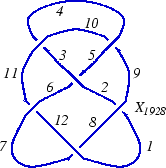
In the "Planar Diagrams" (PD) presentation we present every knot or link diagram by labeling its edges (with natural numbers, 1,...,n, and with increasing labels as we go around each component) and by a list crossings presented as symbols where , , and are the labels of the edges around that crossing, starting from the incoming lower edge and proceeding counterclockwise. Thus for example, the PD presentation of the knot on the right is:
(This of course is the Miller Institute knot, the mirror image of the knot 6_2)
(For In[1] see Setup)
|
In[2]:= PD[v1, v2, ...] represents a planar diagram whose vertices are v1, v2, .... PD also acts as a "type caster", so for example, PD[K] where K is is a named knot (or link) returns the PD presentation of that knot. |
|
In[3]:= X[i,j,k,l] represents a crossing between the edges labeled i, j, k and l starting from the incoming lower strand i and going counterclockwise through j, k and l. The (sometimes ambiguous) orientation of the upper strand is determined by the ordering of {j,l}. |
Thus, for example, let us compute the determinant of the above knot:
In[4]:= K = PD[X[1,9,2,8], X[3,10,4,11], X[5,3,6,2], X[7,1,8,12], X[9,4,10,5], X[11,7,12,6]];
In[5]:= Alexander[K][-1]
Out[5]=
Some further details
For example, we could add an extra "point" on the Miller Institute knot, splitting edge 12 into two pieces, labeled 12 and 13:
At the moment, many of our routines do not know to ignore such ``extra points. But some do:
Hence we can verify that the A2 invariant of the unknot is :


