L11n386: Difference between revisions
From Knot Atlas
Jump to navigationJump to search
DrorsRobot (talk | contribs) No edit summary |
DrorsRobot (talk | contribs) No edit summary |
||
| Line 16: | Line 16: | ||
k = 386 | |
k = 386 | |
||
KnotilusURL = http://srankin.math.uwo.ca/cgi-bin/retrieve.cgi/1,-11,-5,3:-9,8,-10,7:-4,-1,2,5,-6,9,-8,4,11,-2,-3,6,-7,10/goTop.html | |
KnotilusURL = http://srankin.math.uwo.ca/cgi-bin/retrieve.cgi/1,-11,-5,3:-9,8,-10,7:-4,-1,2,5,-6,9,-8,4,11,-2,-3,6,-7,10/goTop.html | |
||
braid_table = <table cellspacing=0 cellpadding=0 border=0> |
braid_table = <table cellspacing=0 cellpadding=0 border=0 style="white-space: pre"> |
||
<tr><td>[[Image:BraidPart3.gif]][[Image:BraidPart0.gif]][[Image:BraidPart3.gif]][[Image:BraidPart0.gif]][[Image:BraidPart1.gif]][[Image:BraidPart0.gif]][[Image:BraidPart0.gif]][[Image:BraidPart0.gif]][[Image:BraidPart0.gif]][[Image:BraidPart0.gif]][[Image:BraidPart0.gif]]</td></tr> |
<tr><td>[[Image:BraidPart3.gif]][[Image:BraidPart0.gif]][[Image:BraidPart3.gif]][[Image:BraidPart0.gif]][[Image:BraidPart1.gif]][[Image:BraidPart0.gif]][[Image:BraidPart0.gif]][[Image:BraidPart0.gif]][[Image:BraidPart0.gif]][[Image:BraidPart0.gif]][[Image:BraidPart0.gif]]</td></tr> |
||
<tr><td>[[Image:BraidPart4.gif]][[Image:BraidPart1.gif]][[Image:BraidPart4.gif]][[Image:BraidPart3.gif]][[Image:BraidPart2.gif]][[Image:BraidPart3.gif]][[Image:BraidPart0.gif]][[Image:BraidPart3.gif]][[Image:BraidPart3.gif]][[Image:BraidPart0.gif]][[Image:BraidPart3.gif]]</td></tr> |
<tr><td>[[Image:BraidPart4.gif]][[Image:BraidPart1.gif]][[Image:BraidPart4.gif]][[Image:BraidPart3.gif]][[Image:BraidPart2.gif]][[Image:BraidPart3.gif]][[Image:BraidPart0.gif]][[Image:BraidPart3.gif]][[Image:BraidPart3.gif]][[Image:BraidPart0.gif]][[Image:BraidPart3.gif]]</td></tr> |
||
| Line 48: | Line 48: | ||
<td align=left><pre style="color: red; border: 0px; padding: 0em"><< KnotTheory`</pre></td> |
<td align=left><pre style="color: red; border: 0px; padding: 0em"><< KnotTheory`</pre></td> |
||
</tr> |
</tr> |
||
<tr valign=top><td colspan=2>Loading KnotTheory` (version of September |
<tr valign=top><td colspan=2>Loading KnotTheory` (version of September 3, 2005, 2:11:43)...</td></tr> |
||
<tr valign=top><td><pre style="color: blue; border: 0px; padding: 0em"><nowiki>In[2]:=</nowiki></pre></td><td><pre style="color: red; border: 0px; padding: 0em"><nowiki>Crossings[Link[11, NonAlternating, 386]]</nowiki></pre></td></tr> |
<tr valign=top><td><pre style="color: blue; border: 0px; padding: 0em"><nowiki>In[2]:=</nowiki></pre></td><td><pre style="color: red; border: 0px; padding: 0em"><nowiki>Crossings[Link[11, NonAlternating, 386]]</nowiki></pre></td></tr> |
||
<tr valign=top><td><pre style="color: blue; border: 0px; padding: 0em"><nowiki>Out[2]= </nowiki></pre></td><td><pre style="color: black; border: 0px; padding: 0em"><nowiki>11</nowiki></pre></td></tr> |
<tr valign=top><td><pre style="color: blue; border: 0px; padding: 0em"><nowiki>Out[2]= </nowiki></pre></td><td><pre style="color: black; border: 0px; padding: 0em"><nowiki>11</nowiki></pre></td></tr> |
||
Latest revision as of 03:13, 3 September 2005
|
|
|
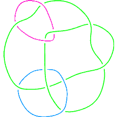
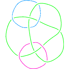
 (Knotscape image) |
See the full Thistlethwaite Link Table (up to 11 crossings). |
Link Presentations
[edit Notes on L11n386's Link Presentations]
| Planar diagram presentation | X6172 X14,7,15,8 X15,1,16,4 X5,12,6,13 X3849 X9,16,10,17 X17,19,18,22 X11,20,12,21 X19,10,20,11 X21,5,22,18 X2,14,3,13 |
| Gauss code | {1, -11, -5, 3}, {-9, 8, -10, 7}, {-4, -1, 2, 5, -6, 9, -8, 4, 11, -2, -3, 6, -7, 10} |
| A Braid Representative |
| ||||
| A Morse Link Presentation | 
|


Polynomial invariants
| Multivariable Alexander Polynomial (in [math]\displaystyle{ u }[/math], [math]\displaystyle{ v }[/math], [math]\displaystyle{ w }[/math], ...) | [math]\displaystyle{ \frac{(u-1) (v-1) (w-1) \left(w^2-w+1\right)}{\sqrt{u} \sqrt{v} w^{3/2}} }[/math] (db) |
| Jones polynomial | [math]\displaystyle{ - q^{-8} +2 q^{-7} -4 q^{-6} +6 q^{-5} -8 q^{-4} +9 q^{-3} -6 q^{-2} +2 q+7 q^{-1} -3 }[/math] (db) |
| Signature | -2 (db) |
| HOMFLY-PT polynomial | [math]\displaystyle{ -z^4 a^6-3 z^2 a^6-a^6 z^{-2} -3 a^6+z^6 a^4+5 z^4 a^4+11 z^2 a^4+4 a^4 z^{-2} +10 a^4-3 z^4 a^2-10 z^2 a^2-5 a^2 z^{-2} -11 a^2+2 z^2+2 z^{-2} +4 }[/math] (db) |
| Kauffman polynomial | [math]\displaystyle{ a^9 z^5-3 a^9 z^3+a^9 z+2 a^8 z^6-5 a^8 z^4+a^8 z^2+3 a^7 z^7-9 a^7 z^5+9 a^7 z^3-5 a^7 z+a^7 z^{-1} +3 a^6 z^8-10 a^6 z^6+14 a^6 z^4-9 a^6 z^2-a^6 z^{-2} +5 a^6+a^5 z^9+2 a^5 z^7-17 a^5 z^5+35 a^5 z^3-22 a^5 z+5 a^5 z^{-1} +5 a^4 z^8-20 a^4 z^6+39 a^4 z^4-34 a^4 z^2-4 a^4 z^{-2} +16 a^4+a^3 z^9-8 a^3 z^5+26 a^3 z^3-26 a^3 z+9 a^3 z^{-1} +2 a^2 z^8-8 a^2 z^6+23 a^2 z^4-32 a^2 z^2-5 a^2 z^{-2} +17 a^2+a z^7-a z^5+3 a z^3-10 a z+5 a z^{-1} +3 z^4-8 z^2-2 z^{-2} +7 }[/math] (db) |
Khovanov Homology
| The coefficients of the monomials [math]\displaystyle{ t^rq^j }[/math] are shown, along with their alternating sums [math]\displaystyle{ \chi }[/math] (fixed [math]\displaystyle{ j }[/math], alternation over [math]\displaystyle{ r }[/math]). |
|
| Integral Khovanov Homology
(db, data source) |
|
Computer Talk
Much of the above data can be recomputed by Mathematica using the package KnotTheory`. See A Sample KnotTheory` Session.
Modifying This Page
| Read me first: Modifying Knot Pages
See/edit the Link Page master template (intermediate). See/edit the Link_Splice_Base (expert). Back to the top. |
|
