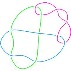
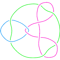
L10a133

L10a132

L10a134

(Knotscape image)	See the full Thistlethwaite Link Table (up to 11 crossings). Visit L10a133 at Knotilus!

Link Presentations

[edit Notes on L10a133's Link Presentations]

Planar diagram presentation	X6172 X12,4,13,3 X14,12,15,11 X20,16,11,15 X8,18,9,17 X16,8,17,7 X18,10,19,9 X10,20,5,19 X2536 X4,14,1,13
Gauss code	{1, -9, 2, -10}, {9, -1, 6, -5, 7, -8}, {3, -2, 10, -3, 4, -6, 5, -7, 8, -4}

A Braid Representative
A Morse Link Presentation

Polynomial invariants

Multivariable Alexander Polynomial (in [math]\displaystyle{ u }[/math], [math]\displaystyle{ v }[/math], [math]\displaystyle{ w }[/math], ...)	[math]\displaystyle{ -\frac{2 t(1) t(3)^2 t(2)^2-2 t(3)^2 t(2)^2-t(1) t(3) t(2)^2+2 t(3) t(2)^2-2 t(1) t(3)^2 t(2)+t(3)^2 t(2)-t(1) t(2)+3 t(1) t(3) t(2)-3 t(3) t(2)+2 t(2)+2 t(1)-2 t(1) t(3)+t(3)-2}{\sqrt{t(1)} t(2) t(3)} }[/math] (db)
Jones polynomial	[math]\displaystyle{ q^{10}-3 q^9+5 q^8-7 q^7+9 q^6-8 q^5+8 q^4-5 q^3+4 q^2-q+1 }[/math] (db)
Signature	4 (db)
HOMFLY-PT polynomial	[math]\displaystyle{ -z^6 a^{-4} -z^6 a^{-6} +z^4 a^{-2} -4 z^4 a^{-4} -3 z^4 a^{-6} +z^4 a^{-8} +4 z^2 a^{-2} -6 z^2 a^{-4} -z^2 a^{-6} +2 z^2 a^{-8} +4 a^{-2} -6 a^{-4} +2 a^{-6} + a^{-2} z^{-2} -2 a^{-4} z^{-2} + a^{-6} z^{-2} }[/math] (db)
Kauffman polynomial	[math]\displaystyle{ z^4 a^{-12} -z^2 a^{-12} +3 z^5 a^{-11} -4 z^3 a^{-11} +4 z^6 a^{-10} -5 z^4 a^{-10} +z^2 a^{-10} +4 z^7 a^{-9} -6 z^5 a^{-9} +4 z^3 a^{-9} +3 z^8 a^{-8} -6 z^6 a^{-8} +9 z^4 a^{-8} -5 z^2 a^{-8} + a^{-8} +z^9 a^{-7} +z^7 a^{-7} -3 z^5 a^{-7} +2 z^3 a^{-7} +4 z^8 a^{-6} -11 z^6 a^{-6} +11 z^4 a^{-6} -2 z^2 a^{-6} + a^{-6} z^{-2} -3 a^{-6} +z^9 a^{-5} -2 z^7 a^{-5} +4 z^5 a^{-5} -9 z^3 a^{-5} +6 z a^{-5} -2 a^{-5} z^{-1} +z^8 a^{-4} -9 z^4 a^{-4} +13 z^2 a^{-4} +2 a^{-4} z^{-2} -8 a^{-4} +z^7 a^{-3} -2 z^5 a^{-3} -3 z^3 a^{-3} +6 z a^{-3} -2 a^{-3} z^{-1} +z^6 a^{-2} -5 z^4 a^{-2} +8 z^2 a^{-2} + a^{-2} z^{-2} -5 a^{-2} }[/math] (db)

Khovanov Homology

The coefficients of the monomials [math]\displaystyle{ t^rq^j }[/math] are shown, along with their alternating sums [math]\displaystyle{ \chi }[/math] (fixed [math]\displaystyle{ j }[/math], alternation over [math]\displaystyle{ r }[/math]).

\   r    \    j   \ -2 -1 0 1 2 3 4 5 6 7 8 χ 21                     1 1 19                   2   -2 17                 3 1   2 15               5 3     -2 13             4 2       2 11           4 5         1 9         4 4           0 7       2 5             3 5     2 3               -1 3   1 4                 3 1                       0 -1 1                     1

Integral Khovanov Homology (db, data source)

[math]\displaystyle{ \dim{\mathcal G}_{2r+i}\operatorname{KH}^r_{\mathbb Z} }[/math] [math]\displaystyle{ i=3 }[/math] [math]\displaystyle{ i=5 }[/math] [math]\displaystyle{ r=-2 }[/math] [math]\displaystyle{ {\mathbb Z} }[/math] [math]\displaystyle{ r=-1 }[/math] [math]\displaystyle{ {\mathbb Z}_2 }[/math] [math]\displaystyle{ {\mathbb Z} }[/math] [math]\displaystyle{ r=0 }[/math] [math]\displaystyle{ {\mathbb Z}^{4} }[/math] [math]\displaystyle{ {\mathbb Z}^{2} }[/math] [math]\displaystyle{ r=1 }[/math] [math]\displaystyle{ {\mathbb Z}^{3}\oplus{\mathbb Z}_2^{2} }[/math] [math]\displaystyle{ {\mathbb Z}^{2} }[/math] [math]\displaystyle{ r=2 }[/math] [math]\displaystyle{ {\mathbb Z}^{5}\oplus{\mathbb Z}_2^{3} }[/math] [math]\displaystyle{ {\mathbb Z}^{4} }[/math] [math]\displaystyle{ r=3 }[/math] [math]\displaystyle{ {\mathbb Z}^{4}\oplus{\mathbb Z}_2^{4} }[/math] [math]\displaystyle{ {\mathbb Z}^{4} }[/math] [math]\displaystyle{ r=4 }[/math] [math]\displaystyle{ {\mathbb Z}^{5}\oplus{\mathbb Z}_2^{4} }[/math] [math]\displaystyle{ {\mathbb Z}^{4} }[/math] [math]\displaystyle{ r=5 }[/math] [math]\displaystyle{ {\mathbb Z}^{2}\oplus{\mathbb Z}_2^{5} }[/math] [math]\displaystyle{ {\mathbb Z}^{5} }[/math] [math]\displaystyle{ r=6 }[/math] [math]\displaystyle{ {\mathbb Z}^{3}\oplus{\mathbb Z}_2^{2} }[/math] [math]\displaystyle{ {\mathbb Z}^{3} }[/math] [math]\displaystyle{ r=7 }[/math] [math]\displaystyle{ {\mathbb Z}\oplus{\mathbb Z}_2^{2} }[/math] [math]\displaystyle{ {\mathbb Z}^{2} }[/math] [math]\displaystyle{ r=8 }[/math] [math]\displaystyle{ {\mathbb Z}_2 }[/math] [math]\displaystyle{ {\mathbb Z} }[/math]

Computer Talk

Much of the above data can be recomputed by Mathematica using the package KnotTheory`. See A Sample KnotTheory` Session.

Modifying This Page

Read me first: Modifying Knot Pages See/edit the Link Page master template (intermediate). See/edit the Link_Splice_Base (expert). Back to the top.

L10a132 L10a134