L11a517

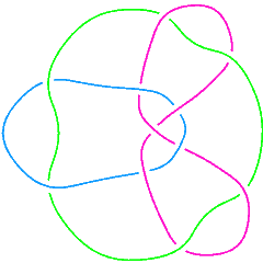
(Knotscape image)

See the full Thistlethwaite Link Table (up to 11 crossings).

Planar diagram presentation	X₈₁₉₂ X_14,4,15,3 X_12,14,7,13 X₂₇₃₈ X_22,10,13,9 X_6,22,1,21 X_20,16,21,15 X_16,5,17,6 X_18,11,19,12 X_10,17,11,18 X_4,19,5,20
Gauss code	{1, -4, 2, -11, 8, -6}, {4, -1, 5, -10, 9, -3}, {3, -2, 7, -8, 10, -9, 11, -7, 6, -5}

A Braid Representative

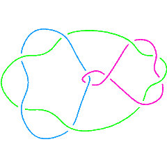
A Morse Link Presentation

Multivariable Alexander Polynomial (in $u$ , $v$ , $w$ , ...)	$- v 2 u 3 - v 2 w 2 u 3 + 2 v w 2 u 3 - w 2 u 3 + v u 3 + 2 v 2 w u 3 -3 v w u 3 + w u 3 + 3 v 2 u 2 + v 2 w 2 u 2 -5 v w 2 u 2 + 3 w 2 u 2 -4 v u 2 -4 v 2 w u 2 + 9 v w u 2 -3 w u 2 -3 v 2 u + 4 v w 2 u -3 w 2 u + 5 v u + 3 v 2 w u -9 v w u + 4 w u - u + v 2 - v w 2 + w 2 -2 v - v 2 w + 3 v w -2 w + 1$ (db)
Jones polynomial	$- q 5 + 4 q 4 -10 q 3 + 18 q 2 -24 q + 29-28 q -1 + 26 q -2 -18 q -3 + 12 q -4 -5 q -5 + q -6$ (db)
Signature	0 (db)
HOMFLY-PT polynomial	$z 8 -2 a 2 z 6 - z 6 a -2 + 5 z 6 + a 4 z 4 -6 a 2 z 4 -3 z 4 a -2 + 11 z 4 + a 4 z 2 -7 a 2 z 2 -4 z 2 a -2 + 10 z 2 + a 4 -4 a 2 - a -2 + 4 + a 4 z -2 -2 a 2 z -2 + z -2$ (db)
Kauffman polynomial	$4 a 2 z 10 + 4 z 10 + 11 a 3 z 9 + 22 a z 9 + 11 z 9 a -1 + 11 a 4 z 8 + 17 a 2 z 8 + 13 z 8 a -2 + 19 z 8 + 5 a 5 z 7 -18 a 3 z 7 -42 a z 7 -10 z 7 a -1 + 9 z 7 a -3 + a 6 z 6 -24 a 4 z 6 -58 a 2 z 6 -21 z 6 a -2 + 4 z 6 a -4 -58 z 6 -8 a 5 z 5 + 3 a 3 z 5 + 20 a z 5 -4 z 5 a -1 -12 z 5 a -3 + z 5 a -5 - a 6 z 4 + 15 a 4 z 4 + 50 a 2 z 4 + 18 z 4 a -2 -4 z 4 a -4 + 56 z 4 + 2 a 5 z 3 + 2 a 3 z 3 + 8 z 3 a -1 + 7 z 3 a -3 - z 3 a -5 -4 a 4 z 2 -21 a 2 z 2 -9 z 2 a -2 + z 2 a -4 -27 z 2 -2 a 3 z -4 a z -3 z a -1 - z a -3 + 3 a 4 + 7 a 2 + 2 a -2 + 7 + 2 a 3 z -1 + 2 a z -1 - a 4 z -2 -2 a 2 z -2 - z -2$ (db)

The coefficients of the monomials

t r q j

are shown, along with their alternating sums

χ

(fixed

j

, alternation over

r

). The squares with yellow highlighting are those on the "critical diagonals", where

j -2 r = s + 1

j -2 r = s -1

, where

s =

0 is the signature of L11a517. Nonzero entries off the critical diagonals (if any exist) are highlighted in red.

$\dim{\mathcal G}_{2r+i}\operatorname{KH}^r_{\mathbb Z}$	$i = -1$	$i = 1$
$r = -6$	${\mathbb Z}$
$r = -5$	${\mathbb Z}^{4}\oplus{\mathbb Z}_2$	${\mathbb Z}$
$r = -4$	${\mathbb Z}^{8}\oplus{\mathbb Z}_2^{4}$	${\mathbb Z}^{4}$
$r = -3$	${\mathbb Z}^{10}\oplus{\mathbb Z}_2^{8}$	${\mathbb Z}^{8}$
$r = -2$	${\mathbb Z}^{16}\oplus{\mathbb Z}_2^{10}$	${\mathbb Z}^{12}$
$r = -1$	${\mathbb Z}^{14}\oplus{\mathbb Z}_2^{14}$	${\mathbb Z}^{14}$
$r = 0$	${\mathbb Z}^{15}\oplus{\mathbb Z}_2^{14}$	${\mathbb Z}^{16}$
$r = 1$	${\mathbb Z}^{11}\oplus{\mathbb Z}_2^{13}$	${\mathbb Z}^{13}$
$r = 2$	${\mathbb Z}^{7}\oplus{\mathbb Z}_2^{11}$	${\mathbb Z}^{11}$
$r = 3$	${\mathbb Z}^{3}\oplus{\mathbb Z}_2^{7}$	${\mathbb Z}^{7}$
$r = 4$	${\mathbb Z}\oplus{\mathbb Z}_2^{3}$	${\mathbb Z}^{3}$
$r = 5$	${\mathbb Z}_2$	${\mathbb Z}$