K11n139: Difference between revisions
DrorsRobot (talk | contribs) No edit summary |
No edit summary |
||
| Line 127: | Line 127: | ||
q t</nowiki></pre></td></tr> |
q t</nowiki></pre></td></tr> |
||
</table> }} |
</table> }} |
||
[http://alansmith12.bravejournal.com/ automobile insurance] |
|||
We have online quotes for automobile insurance, car insurance, breakdown cover, van, motorcycle, home, pet, loans, life and travel insurance. <br> |
|||
Buy your cheap automobile insurance online and save 10%. Looking for low cost bike insurance? You can't lose with Bennetts. Click now to quote and buy online automobile insurance. |
|||
[http://alansmith12.bravejournal.com/ automobile insurance] |
|||
Revision as of 08:40, 30 May 2006
|
|
|
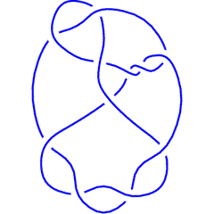
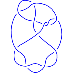
 (Knotscape image) |
See the full Hoste-Thistlethwaite Table of 11 Crossing Knots. |
|
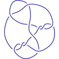
K11n139 is also known as the pretzel knot P(5,3,-3). |
Knot presentations
| Planar diagram presentation | X4251 X12,3,13,4 X16,6,17,5 X14,8,15,7 X9,21,10,20 X11,19,12,18 X2,13,3,14 X6,16,7,15 X17,22,18,1 X19,11,20,10 X21,9,22,8 |
| Gauss code | 1, -7, 2, -1, 3, -8, 4, 11, -5, 10, -6, -2, 7, -4, 8, -3, -9, 6, -10, 5, -11, 9 |
| Dowker-Thistlethwaite code | 4 12 16 14 -20 -18 2 6 -22 -10 -8 |
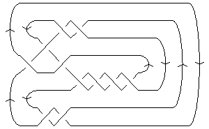
| A Braid Representative | |||||||||
| A Morse Link Presentation | 
|
Three dimensional invariants
|
Four dimensional invariants
|
Polynomial invariants
KnotTheory`, as shown in the (simulated) Mathematica session below. Your input (in red) is realistic; all else should have the same content as in a real mathematica session, but with different formatting. This Mathematica session is also available (albeit only for the knot 5_2) as the notebook PolynomialInvariantsSession.nb.
(The path below may be different on your system, and possibly also the KnotTheory` date)
In[1]:=
|
AppendTo[$Path, "C:/drorbn/projects/KAtlas/"];
<< KnotTheory`
|
Loading KnotTheory` version of August 31, 2006, 11:25:27.5625.
|
In[3]:=
|
K = Knot["K11n139"];
|
In[4]:=
|
Alexander[K][t]
|
KnotTheory::loading: Loading precomputed data in PD4Knots`.
|
Out[4]=
|
In[5]:=
|
Conway[K][z]
|
Out[5]=
|
In[6]:=
|
Alexander[K, 2][t]
|
KnotTheory::credits: The program Alexander[K, r] to compute Alexander ideals was written by Jana Archibald at the University of Toronto in the summer of 2005.
|
Out[6]=
|
In[7]:=
|
{KnotDet[K], KnotSignature[K]}
|
Out[7]=
|
{ 9, 0 } |
In[8]:=
|
Jones[K][q]
|
KnotTheory::loading: Loading precomputed data in Jones4Knots`.
|
Out[8]=
|
In[9]:=
|
HOMFLYPT[K][a, z]
|
KnotTheory::credits: The HOMFLYPT program was written by Scott Morrison.
|
Out[9]=
|
In[10]:=
|
Kauffman[K][a, z]
|
KnotTheory::loading: Loading precomputed data in Kauffman4Knots`.
|
Out[10]=
|
"Similar" Knots (within the Atlas)
Same Alexander/Conway Polynomial: {6_1, 9_46, K11n67, K11n97,}
Same Jones Polynomial (up to mirroring, ): {}
KnotTheory`. Your input (in red) is realistic; all else should have the same content as in a real mathematica session, but with different formatting.
(The path below may be different on your system, and possibly also the KnotTheory` date)
In[1]:=
|
AppendTo[$Path, "C:/drorbn/projects/KAtlas/"];
<< KnotTheory`
|
Loading KnotTheory` version of May 31, 2006, 14:15:20.091.
|
In[3]:=
|
K = Knot["K11n139"];
|
In[4]:=
|
{A = Alexander[K][t], J = Jones[K][q]}
|
KnotTheory::loading: Loading precomputed data in PD4Knots`.
|
KnotTheory::loading: Loading precomputed data in Jones4Knots`.
|
Out[4]=
|
{ , } |
In[5]:=
|
DeleteCases[Select[AllKnots[], (A === Alexander[#][t]) &], K]
|
KnotTheory::loading: Loading precomputed data in DTCode4KnotsTo11`.
|
KnotTheory::credits: The GaussCode to PD conversion was written by Siddarth Sankaran at the University of Toronto in the summer of 2005.
|
Out[5]=
|
{6_1, 9_46, K11n67, K11n97,} |
In[6]:=
|
DeleteCases[
  Select[
    AllKnots[],
    (J === Jones[#][q] || (J /. q -> 1/q) === Jones[#][q]) &
    ],
  K
  ]
|
KnotTheory::loading: Loading precomputed data in Jones4Knots11`.
|
Out[6]=
|
{} |
Vassiliev invariants
| V2 and V3: | (-2, -5) |
| V2,1 through V6,9: |
|
V2,1 through V6,9 were provided by Petr Dunin-Barkowski <barkovs@itep.ru>, Andrey Smirnov <asmirnov@itep.ru>, and Alexei Sleptsov <sleptsov@itep.ru> and uploaded on October 2010 by User:Drorbn. Note that they are normalized differently than V2 and V3.
Khovanov Homology
| The coefficients of the monomials are shown, along with their alternating sums (fixed , alternation over ). The squares with yellow highlighting are those on the "critical diagonals", where or , where 0 is the signature of K11n139. Nonzero entries off the critical diagonals (if any exist) are highlighted in red. |
|
| Integral Khovanov Homology
(db, data source) |
|
Computer Talk
Much of the above data can be recomputed by Mathematica using the package KnotTheory`. See A Sample KnotTheory` Session.
Modifying This Page
| Read me first: Modifying Knot Pages.
See/edit the Hoste-Thistlethwaite Knot Page master template (intermediate). See/edit the Hoste-Thistlethwaite_Splice_Base (expert). Back to the top. |
|
automobile insurance
We have online quotes for automobile insurance, car insurance, breakdown cover, van, motorcycle, home, pet, loans, life and travel insurance.
Buy your cheap automobile insurance online and save 10%. Looking for low cost bike insurance? You can't lose with Bennetts. Click now to quote and buy online automobile insurance.
automobile insurance


