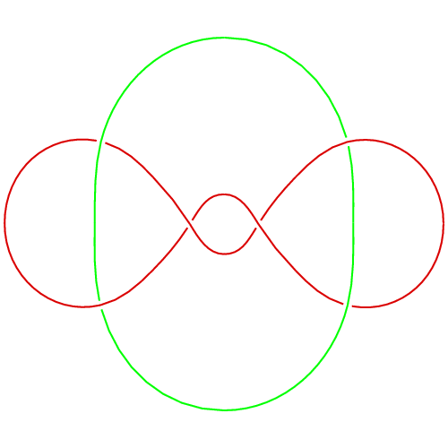
L6a1: Difference between revisions
From Knot Atlas
Jump to navigationJump to search
No edit summary |
No edit summary |
||
| Line 19: | Line 19: | ||
{{Vassiliev Invariants}} |
{{Vassiliev Invariants}} |
||
{{Khovanov Homology|table=<math>\textrm{<table border=1>$\backslash $n<tr align=center>$\backslash $n<td width=40.$\%$><table cellpadding=0 cellspacing=0>$\backslash $n <tr><td>$\backslash \backslash $</td><td>$\&$nbsp;</td><td>r</td></tr>$\backslash $n<tr><td>$\&$nbsp;</td><td>$\&$nbsp;$\backslash \backslash \&$nbsp;</td><td>$\&$nbsp;</td></tr>$\backslash $n<tr><td>j</td><td>$\&$nbsp;</td><td>$\backslash \backslash $</td></tr>$\backslash $n</table></td>$\backslash $n <td width=20.$\%$>0</td ><td width=40.$\%$>$\&$chi;</td></tr>$\backslash $n<tr align=center><td>0</td>}\textrm{<>}\textrm{Which}[\textrm{$\$$Failed}[q,t]\neq 0,\textrm{<td bgcolor=red>}\textrm{<>}\textrm{ToString}[\textrm{c$\$$ |
{{Khovanov Homology|table=<math>\textrm{<table border=1>$\backslash $n<tr align=center>$\backslash $n<td width=40.$\%$><table cellpadding=0 cellspacing=0>$\backslash $n <tr><td>$\backslash \backslash $</td><td>$\&$nbsp;</td><td>r</td></tr>$\backslash $n<tr><td>$\&$nbsp;</td><td>$\&$nbsp;$\backslash \backslash \&$nbsp;</td><td>$\&$nbsp;</td></tr>$\backslash $n<tr><td>j</td><td>$\&$nbsp;</td><td>$\backslash \backslash $</td></tr>$\backslash $n</table></td>$\backslash $n <td width=20.$\%$>0</td ><td width=40.$\%$>$\&$chi;</td></tr>$\backslash $n<tr align=center><td>0</td>}\textrm{<>}\textrm{Which}[\textrm{$\$$Failed}[q,t]\neq 0,\textrm{<td bgcolor=red>}\textrm{<>}\textrm{ToString}[\textrm{c$\$$16963}]\textrm{<>}\textrm{</td>},\neg \textrm{critical$\$$16963}\land \textrm{c$\$$16963}=0,\textrm{<td>$\&$nbsp;</td>}]\textrm{<>}\textrm{<td>$\$$Failed[q, t]</td></tr>$\backslash $n</table>}</math>}} |
||
{{Computer Talk Header}} |
{{Computer Talk Header}} |
||
Revision as of 20:39, 28 August 2005
|
|
|
|
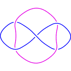
Visit [ L6a1's page] at Knotilus!
Visit 164.html L6a1's page at the original Knot Atlas! |
| L6a1 is in the Rolfsen table of links. |
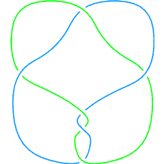
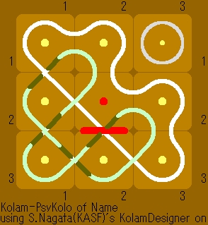 A kolam with two cycles/components[1] |
||
Knot presentations
| Planar diagram presentation | X6172 X10,3,11,4 X12,8,5,7 X8,12,9,11 X2536 X4,9,1,10 |
| Gauss code | {1, -5, 2, -6}, {5, -1, 3, -4, 6, -2, 4, -3} |
Polynomial invariants
| Multivariable Alexander Polynomial (in , , , ...) | (db) |
| Jones polynomial | (db) |
| Signature | -1 (db) |
| HOMFLY-PT polynomial | (db) |
| Kauffman polynomial | (db) |
Vassiliev invariants
| V2 and V3: | (0, ) |
| V2,1 through V6,9: |
|
V2,1 through V6,9 were provided by Petr Dunin-Barkowski <barkovs@itep.ru>, Andrey Smirnov <asmirnov@itep.ru>, and Alexei Sleptsov <sleptsov@itep.ru> and uploaded on October 2010 by User:Drorbn. Note that they are normalized differently than V2 and V3.
Khovanov Homology
| The coefficients of the monomials are shown, along with their alternating sums (fixed , alternation over ). The squares with yellow highlighting are those on the "critical diagonals", where or , where -1 is the signature of L6a1. Nonzero entries off the critical diagonals (if any exist) are highlighted in red. |
|
| Integral Khovanov Homology
(db, data source) |
|
Computer Talk
Much of the above data can be recomputed by Mathematica using the package KnotTheory`. See A Sample KnotTheory` Session.
In[1]:= |
<< KnotTheory` |
Loading KnotTheory` (version of August 17, 2005, 14:44:34)... | |
In[2]:= | Crossings[Knot[L6a1]] |
Out[2]= | 0 |
In[3]:= | PD[Knot[L6a1]] |
Out[3]= | PD[Knot[L6a1]] |
In[4]:= | GaussCode[Knot[L6a1]] |
Out[4]= | GaussCode[PD[Knot[L6a1]]] |
In[5]:= | BR[Knot[L6a1]] |
Out[5]= | BR[Knot[L6a1]] |
In[6]:= | alex = Alexander[Knot[L6a1]][t] |
Out[6]= | 1 |
In[7]:= | Conway[Knot[L6a1]][z] |
Out[7]= | 1 |
In[8]:= | Select[AllKnots[], (alex === Alexander[#][t])&] |
Out[8]= | {Knot[0, 1], Knot[11, NonAlternating, 34], Knot[11, NonAlternating, 42]} |
In[9]:= | {KnotDet[Knot[L6a1]], KnotSignature[Knot[L6a1]]} |
Out[9]= | {1, 0} |
In[10]:= | J=Jones[Knot[L6a1]][q] |
Out[10]= | Sqrt[q] Knot[L6a1] |
In[11]:= | Select[AllKnots[], (J === Jones[#][q] || (J /. q-> 1/q) === Jones[#][q])&] |
Out[11]= | {} |
In[12]:= | A2Invariant[Knot[L6a1]][q] |
Out[12]= | Knot[L6a1] |
In[13]:= | Kauffman[Knot[L6a1]][a, z] |
Out[13]= | 1 |
In[14]:= | {Vassiliev[2][Knot[L6a1]], Vassiliev[3][Knot[L6a1]]} |
Out[14]= | {0, 0} |
In[15]:= | Kh[Knot[L6a1]][q, t] |
Out[15]= | $Failed[q, t] |

![{\displaystyle {\textrm {If}}[{\textrm {AlternatingQ}}({\textrm {Knot}}({\textrm {L6a1}})),a,n]}](https://wikimedia.org/api/rest_v1/media/math/render/svg/5a0039fcc2b4f3ea1990a56818ef46ec9b442d9a)

