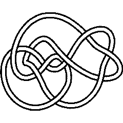
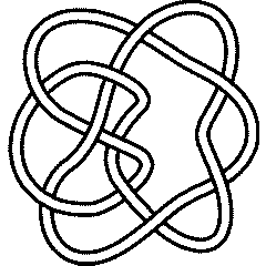
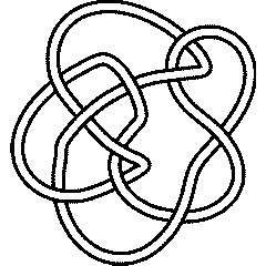
10 86
|
|
|

|
Visit 10 86's page at the Knot Server (KnotPlot driven, includes 3D interactive images!)
Visit 10 86's page at Knotilus! Visit 10 86's page at the original Knot Atlas! |
10 86 Quick Notes |
Warning. There is a mixup in the original (1976) Rolfsen table between the pictures and the invariants of the knots 10_83 and 10_86. That mixup lead to a similar mixup here. In the new (2003) edition of Rolfsen's book the mixup was corrected and on August 17, 2004, it was corrected here (actually in Dror's original Knot Atlas) consistently with Rolfsen's correction. In the years between 1976 and 2003 other authors fixed the problem in different ways and our enumeration here may be different than theirs. Dror would like to thank Z-X. Tao for telling him about the (now corrected) mixup here and A. Stoimenow for telling him about the mixup in Rolfsen's original table.
Knot presentations
| Planar diagram presentation | X6271 X16,8,17,7 X8394 X2,15,3,16 X14,5,15,6 X4,9,5,10 X20,14,1,13 X10,20,11,19 X18,12,19,11 X12,18,13,17 |
| Gauss code | 1, -4, 3, -6, 5, -1, 2, -3, 6, -8, 9, -10, 7, -5, 4, -2, 10, -9, 8, -7 |
| Dowker-Thistlethwaite code | 6 8 14 16 4 18 20 2 12 10 |
| Conway Notation | [.31.2] |
Three dimensional invariants
|
Four dimensional invariants
|
Polynomial invariants
A1 Invariants.
| Weight | Invariant |
|---|---|
| 1 | |
| 2 | |
| 3 | |
| 4 | |
| 5 |
A2 Invariants.
| Weight | Invariant |
|---|---|
| 1,0 | |
| 1,1 | |
| 2,0 |
A3 Invariants.
| Weight | Invariant |
|---|---|
| 0,1,0 | |
| 1,0,0 |
A4 Invariants.
| Weight | Invariant |
|---|---|
| 0,1,0,0 | |
| 1,0,0,0 |
B2 Invariants.
| Weight | Invariant |
|---|---|
| 0,1 | |
| 1,0 |
D4 Invariants.
| Weight | Invariant |
|---|---|
| 1,0,0,0 |
G2 Invariants.
| Weight | Invariant |
|---|---|
| 1,0 |
.
KnotTheory`, as shown in the (simulated) Mathematica session below. Your input (in red) is realistic; all else should have the same content as in a real mathematica session, but with different formatting. This Mathematica session is also available (albeit only for the knot 5_2) as the notebook PolynomialInvariantsSession.nb.
(The path below may be different on your system, and possibly also the KnotTheory` date)
In[1]:=
|
AppendTo[$Path, "C:/drorbn/projects/KAtlas/"];
<< KnotTheory`
|
Loading KnotTheory` version of August 31, 2006, 11:25:27.5625.
|
In[3]:=
|
K = Knot["10 86"];
|
In[4]:=
|
Alexander[K][t]
|
KnotTheory::loading: Loading precomputed data in PD4Knots`.
|
Out[4]=
|
In[5]:=
|
Conway[K][z]
|
Out[5]=
|
In[6]:=
|
Alexander[K, 2][t]
|
KnotTheory::credits: The program Alexander[K, r] to compute Alexander ideals was written by Jana Archibald at the University of Toronto in the summer of 2005.
|
Out[6]=
|
In[7]:=
|
{KnotDet[K], KnotSignature[K]}
|
Out[7]=
|
{ 85, 0 } |
In[8]:=
|
Jones[K][q]
|
KnotTheory::loading: Loading precomputed data in Jones4Knots`.
|
Out[8]=
|
In[9]:=
|
HOMFLYPT[K][a, z]
|
KnotTheory::credits: The HOMFLYPT program was written by Scott Morrison.
|
Out[9]=
|
In[10]:=
|
Kauffman[K][a, z]
|
KnotTheory::loading: Loading precomputed data in Kauffman4Knots`.
|
Out[10]=
|
Vassiliev invariants
| V2 and V3: | (-1, -1) |
| V2,1 through V6,9: |
|
V2,1 through V6,9 were provided by Petr Dunin-Barkowski <barkovs@itep.ru>, Andrey Smirnov <asmirnov@itep.ru>, and Alexei Sleptsov <sleptsov@itep.ru> and uploaded on October 2010 by User:Drorbn. Note that they are normalized differently than V2 and V3.
Khovanov Homology
The coefficients of the monomials are shown, along with their alternating sums (fixed , alternation over ). The squares with yellow highlighting are those on the "critical diagonals", where or , where 0 is the signature of 10 86. Nonzero entries off the critical diagonals (if any exist) are highlighted in red.
|
-4 | -3 | -2 | -1 | 0 | 1 | 2 | 3 | 4 | 5 | 6 | χ | |||||||||
| 13 | 1 | 1 | |||||||||||||||||||
| 11 | 2 | -2 | |||||||||||||||||||
| 9 | 4 | 1 | 3 | ||||||||||||||||||
| 7 | 6 | 2 | -4 | ||||||||||||||||||
| 5 | 7 | 4 | 3 | ||||||||||||||||||
| 3 | 7 | 6 | -1 | ||||||||||||||||||
| 1 | 7 | 7 | 0 | ||||||||||||||||||
| -1 | 5 | 8 | 3 | ||||||||||||||||||
| -3 | 3 | 6 | -3 | ||||||||||||||||||
| -5 | 1 | 5 | 4 | ||||||||||||||||||
| -7 | 3 | -3 | |||||||||||||||||||
| -9 | 1 | 1 |
Computer Talk
Much of the above data can be recomputed by Mathematica using the package KnotTheory`. See A Sample KnotTheory` Session.
In[1]:= |
<< KnotTheory` |
Loading KnotTheory` (version of August 17, 2005, 14:44:34)... | |
In[2]:= | Crossings[Knot[10, 86]] |
Out[2]= | 10 |
In[3]:= | PD[Knot[10, 86]] |
Out[3]= | PD[X[6, 2, 7, 1], X[16, 8, 17, 7], X[8, 3, 9, 4], X[2, 15, 3, 16],X[14, 5, 15, 6], X[4, 9, 5, 10], X[20, 14, 1, 13], X[10, 20, 11, 19],X[18, 12, 19, 11], X[12, 18, 13, 17]] |
In[4]:= | GaussCode[Knot[10, 86]] |
Out[4]= | GaussCode[1, -4, 3, -6, 5, -1, 2, -3, 6, -8, 9, -10, 7, -5, 4, -2, 10, -9, 8, -7] |
In[5]:= | BR[Knot[10, 86]] |
Out[5]= | BR[4, {-1, -1, 2, -1, 2, -1, 2, 2, 3, -2, 3}] |
In[6]:= | alex = Alexander[Knot[10, 86]][t] |
Out[6]= | 2 9 19 2 3 |
In[7]:= | Conway[Knot[10, 86]][z] |
Out[7]= | 2 4 6 1 - z - 3 z - 2 z |
In[8]:= | Select[AllKnots[], (alex === Alexander[#][t])&] |
Out[8]= | {Knot[10, 86], Knot[11, Alternating, 190]} |
In[9]:= | {KnotDet[Knot[10, 86]], KnotSignature[Knot[10, 86]]} |
Out[9]= | {85, 0} |
In[10]:= | J=Jones[Knot[10, 86]][q] |
Out[10]= | -4 4 8 11 2 3 4 5 6 |
In[11]:= | Select[AllKnots[], (J === Jones[#][q] || (J /. q-> 1/q) === Jones[#][q])&] |
Out[11]= | {Knot[10, 60], Knot[10, 86]} |
In[12]:= | A2Invariant[Knot[10, 86]][q] |
Out[12]= | -12 2 -8 -6 2 4 2 6 8 10 |
In[13]:= | Kauffman[Knot[10, 86]][a, z] |
Out[13]= | 2 2 2-4 2 2 z 4 z 3 z 2 2 z 2 z 6 z |
In[14]:= | {Vassiliev[2][Knot[10, 86]], Vassiliev[3][Knot[10, 86]]} |
Out[14]= | {0, -1} |
In[15]:= | Kh[Knot[10, 86]][q, t] |
Out[15]= | 8 1 3 1 5 3 6 5 |


