K11a57

K11a56

K11a58

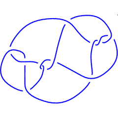
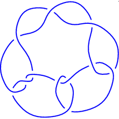
	Visit K11a57's page at Knotilus! Visit K11a57's page at the original Knot Atlas!
	K11a57 Quick Notes

K11a57 Further Notes and Views

Knot presentations

Planar diagram presentation	X4251 X8493 X16,6,17,5 X2837 X20,9,21,10 X22,11,1,12 X18,13,19,14 X6,16,7,15 X12,17,13,18 X14,19,15,20 X10,21,11,22
Gauss code	1, -4, 2, -1, 3, -8, 4, -2, 5, -11, 6, -9, 7, -10, 8, -3, 9, -7, 10, -5, 11, -6
Dowker-Thistlethwaite code	4 8 16 2 20 22 18 6 12 14 10
Conway Notation	[3,3,21,2]

Three dimensional invariants

Symmetry type Reversible Unknotting number [math]\displaystyle{ \{1,2\} }[/math] 3-genus 4 Bridge index 4 Super bridge index Missing Nakanishi index Missing Maximal Thurston-Bennequin number Data:K11a57/ThurstonBennequinNumber Hyperbolic Volume 14.7354 A-Polynomial See Data:K11a57/A-polynomial

[edit Notes for K11a57's three dimensional invariants]

Four dimensional invariants

Smooth 4 genus Missing Topological 4 genus Missing Concordance genus [math]\displaystyle{ [2,4] }[/math] Rasmussen s-Invariant 2

[edit Notes for K11a57's four dimensional invariants]

Polynomial invariants

Alexander polynomial	[math]\displaystyle{ -t^4+5 t^3-12 t^2+20 t-23+20 t^{-1} -12 t^{-2} +5 t^{-3} - t^{-4} }[/math]
Conway polynomial	[math]\displaystyle{ -z^8-3 z^6-2 z^4+z^2+1 }[/math]
2nd Alexander ideal (db, data sources)	[math]\displaystyle{ \left\{t^2-t+1\right\} }[/math]
Determinant and Signature	{ 99, -2 }
Jones polynomial	[math]\displaystyle{ -q^4+2 q^3-5 q^2+10 q-12+16 q^{-1} -16 q^{-2} +14 q^{-3} -12 q^{-4} +7 q^{-5} -3 q^{-6} + q^{-7} }[/math]
HOMFLY-PT polynomial (db, data sources)	[math]\displaystyle{ -a^2 z^8+a^4 z^6-6 a^2 z^6+2 z^6+4 a^4 z^4-15 a^2 z^4-z^4 a^{-2} +10 z^4+6 a^4 z^2-19 a^2 z^2-4 z^2 a^{-2} +18 z^2+3 a^4-10 a^2-4 a^{-2} +12 }[/math]
Kauffman polynomial (db, data sources)	[math]\displaystyle{ a^2 z^{10}+z^{10}+4 a^3 z^9+6 a z^9+2 z^9 a^{-1} +8 a^4 z^8+10 a^2 z^8+2 z^8 a^{-2} +4 z^8+9 a^5 z^7+4 a^3 z^7-9 a z^7-3 z^7 a^{-1} +z^7 a^{-3} +6 a^6 z^6-12 a^4 z^6-31 a^2 z^6-8 z^6 a^{-2} -21 z^6+3 a^7 z^5-16 a^5 z^5-29 a^3 z^5-14 a z^5-9 z^5 a^{-1} -5 z^5 a^{-3} +a^8 z^4-6 a^6 z^4+6 a^4 z^4+30 a^2 z^4+11 z^4 a^{-2} +28 z^4-2 a^7 z^3+16 a^5 z^3+35 a^3 z^3+29 a z^3+20 z^3 a^{-1} +8 z^3 a^{-3} -a^8 z^2+3 a^6 z^2-2 a^4 z^2-22 a^2 z^2-8 z^2 a^{-2} -24 z^2-6 a^5 z-16 a^3 z-17 a z-11 z a^{-1} -4 z a^{-3} +3 a^4+10 a^2+4 a^{-2} +12 }[/math]
The A2 invariant	[math]\displaystyle{ q^{20}-q^{18}+3 q^{16}-q^{14}-q^{12}-6 q^8+q^6-3 q^4+4 q^2+5+2 q^{-2} +4 q^{-4} -2 q^{-6} - q^{-8} - q^{-10} - q^{-12} }[/math]
The G2 invariant	[math]\displaystyle{ q^{114}-2 q^{112}+4 q^{110}-6 q^{108}+6 q^{106}-5 q^{104}+9 q^{100}-19 q^{98}+29 q^{96}-38 q^{94}+35 q^{92}-22 q^{90}-5 q^{88}+49 q^{86}-87 q^{84}+115 q^{82}-119 q^{80}+82 q^{78}-16 q^{76}-81 q^{74}+178 q^{72}-232 q^{70}+223 q^{68}-133 q^{66}-4 q^{64}+156 q^{62}-252 q^{60}+268 q^{58}-177 q^{56}+20 q^{54}+136 q^{52}-227 q^{50}+204 q^{48}-65 q^{46}-111 q^{44}+242 q^{42}-274 q^{40}+170 q^{38}+19 q^{36}-243 q^{34}+375 q^{32}-397 q^{30}+265 q^{28}-43 q^{26}-210 q^{24}+377 q^{22}-414 q^{20}+315 q^{18}-126 q^{16}-99 q^{14}+262 q^{12}-302 q^{10}+229 q^8-54 q^6-119 q^4+242 q^2-219+99 q^{-2} +86 q^{-4} -233 q^{-6} +304 q^{-8} -242 q^{-10} +84 q^{-12} +106 q^{-14} -243 q^{-16} +304 q^{-18} -249 q^{-20} +121 q^{-22} +17 q^{-24} -131 q^{-26} +174 q^{-28} -164 q^{-30} +104 q^{-32} -36 q^{-34} -21 q^{-36} +51 q^{-38} -59 q^{-40} +45 q^{-42} -26 q^{-44} +8 q^{-46} +2 q^{-48} -9 q^{-50} +7 q^{-52} -6 q^{-54} +4 q^{-56} - q^{-58} + q^{-60} }[/math]

Further Quantum Invariants

K11a57 Quantum Invariants.

Computer Talk

The above data is available with the Mathematica package KnotTheory`, as shown in the (simulated) Mathematica session below. Your input (in red) is realistic; all else should have the same content as in a real mathematica session, but with different formatting. This Mathematica session is also available (albeit only for the knot 5_2) as the notebook PolynomialInvariantsSession.nb.

(The path below may be different on your system, and possibly also the KnotTheory` date)

In[1]:=

AppendTo[$Path, "C:/drorbn/projects/KAtlas/"]; << KnotTheory`

Loading KnotTheory` version of August 31, 2006, 11:25:27.5625. Read more at http://katlas.math.toronto.edu/wiki/KnotTheory.

In[3]:=

K = Knot["K11a57"];

In[4]:=

Alexander[K][t]

KnotTheory::loading: Loading precomputed data in PD4Knots`.

Out[4]=

[math]\displaystyle{ -t^4+5 t^3-12 t^2+20 t-23+20 t^{-1} -12 t^{-2} +5 t^{-3} - t^{-4} }[/math]

In[5]:=

Conway[K][z]

Out[5]=

[math]\displaystyle{ -z^8-3 z^6-2 z^4+z^2+1 }[/math]

In[6]:=

Alexander[K, 2][t]

KnotTheory::credits: The program Alexander[K, r] to compute Alexander ideals was written by Jana Archibald at the University of Toronto in the summer of 2005.

Out[6]=

[math]\displaystyle{ \left\{t^2-t+1\right\} }[/math]

In[7]:=

{KnotDet[K], KnotSignature[K]}

Out[7]=

{ 99, -2 }

In[8]:=

Jones[K][q]

KnotTheory::loading: Loading precomputed data in Jones4Knots`.

Out[8]=

[math]\displaystyle{ -q^4+2 q^3-5 q^2+10 q-12+16 q^{-1} -16 q^{-2} +14 q^{-3} -12 q^{-4} +7 q^{-5} -3 q^{-6} + q^{-7} }[/math]

In[9]:=

HOMFLYPT[K][a, z]

KnotTheory::credits: The HOMFLYPT program was written by Scott Morrison.

Out[9]=

[math]\displaystyle{ -a^2 z^8+a^4 z^6-6 a^2 z^6+2 z^6+4 a^4 z^4-15 a^2 z^4-z^4 a^{-2} +10 z^4+6 a^4 z^2-19 a^2 z^2-4 z^2 a^{-2} +18 z^2+3 a^4-10 a^2-4 a^{-2} +12 }[/math]

In[10]:=

Kauffman[K][a, z]

KnotTheory::loading: Loading precomputed data in Kauffman4Knots`.

Out[10]=

[math]\displaystyle{ a^2 z^{10}+z^{10}+4 a^3 z^9+6 a z^9+2 z^9 a^{-1} +8 a^4 z^8+10 a^2 z^8+2 z^8 a^{-2} +4 z^8+9 a^5 z^7+4 a^3 z^7-9 a z^7-3 z^7 a^{-1} +z^7 a^{-3} +6 a^6 z^6-12 a^4 z^6-31 a^2 z^6-8 z^6 a^{-2} -21 z^6+3 a^7 z^5-16 a^5 z^5-29 a^3 z^5-14 a z^5-9 z^5 a^{-1} -5 z^5 a^{-3} +a^8 z^4-6 a^6 z^4+6 a^4 z^4+30 a^2 z^4+11 z^4 a^{-2} +28 z^4-2 a^7 z^3+16 a^5 z^3+35 a^3 z^3+29 a z^3+20 z^3 a^{-1} +8 z^3 a^{-3} -a^8 z^2+3 a^6 z^2-2 a^4 z^2-22 a^2 z^2-8 z^2 a^{-2} -24 z^2-6 a^5 z-16 a^3 z-17 a z-11 z a^{-1} -4 z a^{-3} +3 a^4+10 a^2+4 a^{-2} +12 }[/math]

Vassiliev invariants

V2 and V3:

(1, 3)

V2,1 through V6,9:

V2,1 V3,1 V4,1 V4,2 V4,3 V5,1 V5,2 V5,3 V5,4 V6,1 V6,2 V6,3 V6,4 V6,5 V6,6 V6,7 V6,8 V6,9 [math]\displaystyle{ 4 }[/math] [math]\displaystyle{ 24 }[/math] [math]\displaystyle{ 8 }[/math] [math]\displaystyle{ \frac{14}{3} }[/math] [math]\displaystyle{ \frac{58}{3} }[/math] [math]\displaystyle{ 96 }[/math] [math]\displaystyle{ 80 }[/math] [math]\displaystyle{ -64 }[/math] [math]\displaystyle{ 24 }[/math] [math]\displaystyle{ \frac{32}{3} }[/math] [math]\displaystyle{ 288 }[/math] [math]\displaystyle{ \frac{56}{3} }[/math] [math]\displaystyle{ \frac{232}{3} }[/math] [math]\displaystyle{ \frac{19231}{30} }[/math] [math]\displaystyle{ \frac{1258}{15} }[/math] [math]\displaystyle{ \frac{13622}{45} }[/math] [math]\displaystyle{ \frac{929}{18} }[/math] [math]\displaystyle{ \frac{511}{30} }[/math]

V_2,1 through V_6,9 were provided by Petr Dunin-Barkowski <barkovs@itep.ru>, Andrey Smirnov <asmirnov@itep.ru>, and Alexei Sleptsov <sleptsov@itep.ru> and uploaded on October 2010 by User:Drorbn. Note that they are normalized differently than V₂ and V₃.

Khovanov Homology

The coefficients of the monomials [math]\displaystyle{ t^rq^j }[/math] are shown, along with their alternating sums [math]\displaystyle{ \chi }[/math] (fixed [math]\displaystyle{ j }[/math], alternation over [math]\displaystyle{ r }[/math]). The squares with yellow highlighting are those on the "critical diagonals", where [math]\displaystyle{ j-2r=s+1 }[/math] or [math]\displaystyle{ j-2r=s-1 }[/math], where [math]\displaystyle{ s= }[/math]-2 is the signature of K11a57. Nonzero entries off the critical diagonals (if any exist) are highlighted in red.

\   r    \    j   \ -6 -5 -4 -3 -2 -1 0 1 2 3 4 5 χ 9                       1 -1 7                     1   1 5                   4 1   -3 3                 6 1     5 1               6 4       -2 -1             10 6         4 -3           7 7           0 -5         7 9             -2 -7       5 7               2 -9     2 7                 -5 -11   1 5                   4 -13   2                     -2 -15 1                       1

Integral Khovanov Homology (db, data source)

[math]\displaystyle{ \dim{\mathcal G}_{2r+i}\operatorname{KH}^r_{\mathbb Z} }[/math] [math]\displaystyle{ i=-3 }[/math] [math]\displaystyle{ i=-1 }[/math] [math]\displaystyle{ r=-6 }[/math] [math]\displaystyle{ {\mathbb Z} }[/math] [math]\displaystyle{ r=-5 }[/math] [math]\displaystyle{ {\mathbb Z}^{2}\oplus{\mathbb Z}_2 }[/math] [math]\displaystyle{ {\mathbb Z} }[/math] [math]\displaystyle{ r=-4 }[/math] [math]\displaystyle{ {\mathbb Z}^{5}\oplus{\mathbb Z}_2^{2} }[/math] [math]\displaystyle{ {\mathbb Z}^{2} }[/math] [math]\displaystyle{ r=-3 }[/math] [math]\displaystyle{ {\mathbb Z}^{7}\oplus{\mathbb Z}_2^{5} }[/math] [math]\displaystyle{ {\mathbb Z}^{5} }[/math] [math]\displaystyle{ r=-2 }[/math] [math]\displaystyle{ {\mathbb Z}^{7}\oplus{\mathbb Z}_2^{7} }[/math] [math]\displaystyle{ {\mathbb Z}^{7} }[/math] [math]\displaystyle{ r=-1 }[/math] [math]\displaystyle{ {\mathbb Z}^{9}\oplus{\mathbb Z}_2^{7} }[/math] [math]\displaystyle{ {\mathbb Z}^{7} }[/math] [math]\displaystyle{ r=0 }[/math] [math]\displaystyle{ {\mathbb Z}^{7}\oplus{\mathbb Z}_2^{9} }[/math] [math]\displaystyle{ {\mathbb Z}^{10} }[/math] [math]\displaystyle{ r=1 }[/math] [math]\displaystyle{ {\mathbb Z}^{6}\oplus{\mathbb Z}_2^{6} }[/math] [math]\displaystyle{ {\mathbb Z}^{6} }[/math] [math]\displaystyle{ r=2 }[/math] [math]\displaystyle{ {\mathbb Z}^{4}\oplus{\mathbb Z}_2^{6} }[/math] [math]\displaystyle{ {\mathbb Z}^{6} }[/math] [math]\displaystyle{ r=3 }[/math] [math]\displaystyle{ {\mathbb Z}\oplus{\mathbb Z}_2^{4} }[/math] [math]\displaystyle{ {\mathbb Z}^{4} }[/math] [math]\displaystyle{ r=4 }[/math] [math]\displaystyle{ {\mathbb Z}\oplus{\mathbb Z}_2 }[/math] [math]\displaystyle{ {\mathbb Z} }[/math] [math]\displaystyle{ r=5 }[/math] [math]\displaystyle{ {\mathbb Z}_2 }[/math] [math]\displaystyle{ {\mathbb Z} }[/math]

Computer Talk

Much of the above data can be recomputed by Mathematica using the package KnotTheory`. See A Sample KnotTheory` Session.

[math]\displaystyle{ \textrm{Include}(\textrm{ColouredJonesM.mhtml}) }[/math]

In[1]:=	<< KnotTheory`
Loading KnotTheory` (version of August 17, 2005, 14:44:34)...
In[2]:=	Crossings[Knot[11, Alternating, 57]]
Out[2]=	11
In[3]:=	PD[Knot[11, Alternating, 57]]
Out[3]=	PD[X[4, 2, 5, 1], X[8, 4, 9, 3], X[16, 6, 17, 5], X[2, 8, 3, 7], X[20, 9, 21, 10], X[22, 11, 1, 12], X[18, 13, 19, 14], X[6, 16, 7, 15], X[12, 17, 13, 18], X[14, 19, 15, 20], X[10, 21, 11, 22]]
In[4]:=	GaussCode[Knot[11, Alternating, 57]]
Out[4]=	GaussCode[1, -4, 2, -1, 3, -8, 4, -2, 5, -11, 6, -9, 7, -10, 8, -3, 9, -7, 10, -5, 11, -6]
In[5]:=	BR[Knot[11, Alternating, 57]]
Out[5]=	BR[Knot[11, Alternating, 57]]
In[6]:=	alex = Alexander[Knot[11, Alternating, 57]][t]
Out[6]=	-4 5 12 20 2 3 4 -23 - t + -- - -- + -- + 20 t - 12 t + 5 t - t 3 2 t t t
In[7]:=	Conway[Knot[11, Alternating, 57]][z]
Out[7]=	2 4 6 8 1 + z - 2 z - 3 z - z
In[8]:=	Select[AllKnots[], (alex === Alexander[#][t])&]
Out[8]=	{Knot[11, Alternating, 57], Knot[11, Alternating, 108], Knot[11, Alternating, 139], Knot[11, Alternating, 231]}
In[9]:=	{KnotDet[Knot[11, Alternating, 57]], KnotSignature[Knot[11, Alternating, 57]]}
Out[9]=	{99, -2}
In[10]:=	J=Jones[Knot[11, Alternating, 57]][q]
Out[10]=	-7 3 7 12 14 16 16 2 3 4 -12 + q - -- + -- - -- + -- - -- + -- + 10 q - 5 q + 2 q - q 6 5 4 3 2 q q q q q q
In[11]:=	Select[AllKnots[], (J === Jones[#][q] || (J /. q-> 1/q) === Jones[#][q])&]
Out[11]=	{Knot[11, Alternating, 57], Knot[11, Alternating, 231]}
In[12]:=	A2Invariant[Knot[11, Alternating, 57]][q]
Out[12]=	-20 -18 3 -14 -12 6 -6 3 4 2 5 + q - q + --- - q - q - -- + q - -- + -- + 2 q + 16 8 4 2 q q q q 4 6 8 10 12 4 q - 2 q - q - q - q
In[13]:=	Kauffman[Knot[11, Alternating, 57]][a, z]
Out[13]=	4 2 4 4 z 11 z 3 5 12 + -- + 10 a + 3 a - --- - ---- - 17 a z - 16 a z - 6 a z - 2 3 a a a 2 3 3 2 8 z 2 2 4 2 6 2 8 2 8 z 20 z 24 z - ---- - 22 a z - 2 a z + 3 a z - a z + ---- + ----- + 2 3 a a a 4 3 3 3 5 3 7 3 4 11 z 2 4 29 a z + 35 a z + 16 a z - 2 a z + 28 z + ----- + 30 a z + 2 a 5 5 4 4 6 4 8 4 5 z 9 z 5 3 5 6 a z - 6 a z + a z - ---- - ---- - 14 a z - 29 a z - 3 a a 6 5 5 7 5 6 8 z 2 6 4 6 6 6 16 a z + 3 a z - 21 z - ---- - 31 a z - 12 a z + 6 a z + 2 a 7 7 8 z 3 z 7 3 7 5 7 8 2 z 2 8 -- - ---- - 9 a z + 4 a z + 9 a z + 4 z + ---- + 10 a z + 3 a 2 a a 9 4 8 2 z 9 3 9 10 2 10 8 a z + ---- + 6 a z + 4 a z + z + a z a
In[14]:=	{Vassiliev[2][Knot[11, Alternating, 57]], Vassiliev[3][Knot[11, Alternating, 57]]}
Out[14]=	{0, 3}
In[15]:=	Kh[Knot[11, Alternating, 57]][q, t]
Out[15]=	7 10 1 2 1 5 2 7 5 -- + -- + ------ + ------ + ------ + ------ + ----- + ----- + ----- + 3 q 15 6 13 5 11 5 11 4 9 4 9 3 7 3 q q t q t q t q t q t q t q t 7 7 9 7 6 t 2 3 2 ----- + ----- + ---- + ---- + --- + 6 q t + 4 q t + 6 q t + 7 2 5 2 5 3 q q t q t q t q t 3 3 5 3 5 4 7 4 9 5 q t + 4 q t + q t + q t + q t