T(5,2)
|
[[Image:T(3,2).{{{ext}}}|80px|link=T(3,2)]] |
[[Image:T(7,2).{{{ext}}}|80px|link=T(7,2)]] |

|
Visit T(5,2)'s page at Knotilus!
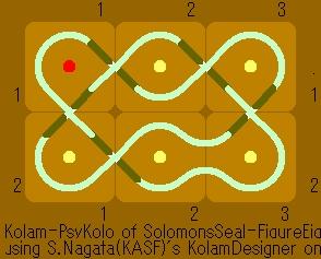
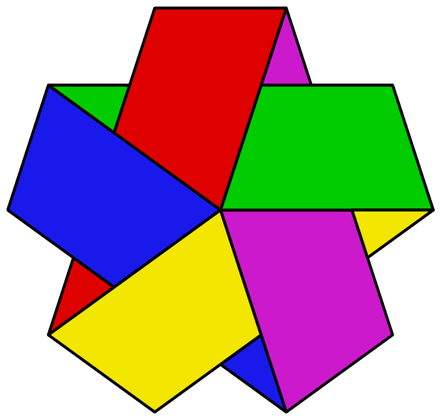
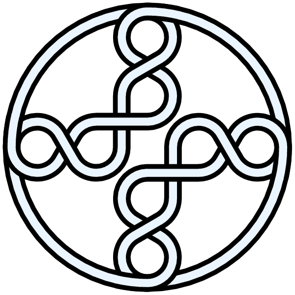
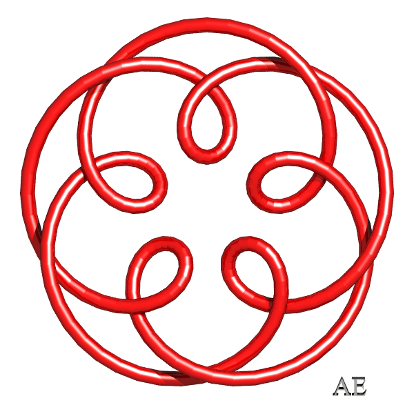
Visit T(5,2)'s page at the original Knot Atlas! An interlaced pentagram, this is known variously as the "Cinquefoil Knot", after certain herbs and shrubs of the rose family which have 5-lobed leaves and 5-petaled flowers (see e.g. [4]), as the "Pentafoil Knot" (visit Bert Jagers' pentafoil page), as the "Double Overhand Knot", as 5_1, or finally as the torus knot T(5,2). When taken off the post the strangle knot (hitch) of practical knot tying deforms to 5_1 |
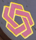
 The VISA Interlink Logo [1] |
 Version of the US bicentennial emblem | |
 A pentagonal table by Bob Mackay [2] |
||
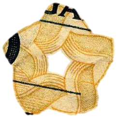
 Partial view of US bicentennial logo on a shirt seen in Lisboa [3] | ||
This sentence was last edited by Dror. Sometime later, Scott added this sentence.
Knot presentations
| Planar diagram presentation | X3948 X9,5,10,4 X5,1,6,10 X1726 X7382 |
| Gauss code | {-4, 5, -1, 2, -3, 4, -5, 1, -2, 3} |
| Dowker-Thistlethwaite code | 6 8 10 2 4 |
Polynomial invariants
KnotTheory`, as shown in the (simulated) Mathematica session below. Your input (in red) is realistic; all else should have the same content as in a real mathematica session, but with different formatting. This Mathematica session is also available (albeit only for the knot 5_2) as the notebook PolynomialInvariantsSession.nb.
(The path below may be different on your system, and possibly also the KnotTheory` date)
In[1]:=
|
AppendTo[$Path, "C:/drorbn/projects/KAtlas/"];
<< KnotTheory`
|
Loading KnotTheory` version of August 31, 2006, 11:25:27.5625.
|
In[3]:=
|
K = Knot["T(5,2)"];
|
In[4]:=
|
Alexander[K][t]
|
KnotTheory::loading: Loading precomputed data in PD4Knots`.
|
Out[4]=
|
In[5]:=
|
Conway[K][z]
|
Out[5]=
|
In[6]:=
|
Alexander[K, 2][t]
|
KnotTheory::credits: The program Alexander[K, r] to compute Alexander ideals was written by Jana Archibald at the University of Toronto in the summer of 2005.
|
Out[6]=
|
In[7]:=
|
{KnotDet[K], KnotSignature[K]}
|
Out[7]=
|
{ 5, 4 } |
In[8]:=
|
Jones[K][q]
|
KnotTheory::loading: Loading precomputed data in Jones4Knots`.
|
Out[8]=
|
In[9]:=
|
HOMFLYPT[K][a, z]
|
KnotTheory::credits: The HOMFLYPT program was written by Scott Morrison.
|
Out[9]=
|
In[10]:=
|
Kauffman[K][a, z]
|
KnotTheory::loading: Loading precomputed data in Kauffman4Knots`.
|
Out[10]=
|
Vassiliev invariants
| V2 and V3 | {0, 5} |
Khovanov Homology
The coefficients of the monomials are shown, along with their alternating sums (fixed , alternation over ). The squares with yellow highlighting are those on the "critical diagonals", where or , where 4 is the signature of T(5,2). Nonzero entries off the critical diagonals (if any exist) are highlighted in red.
|
0 | 1 | 2 | 3 | 4 | 5 | χ | |||||||||
| 15 | 1 | -1 | ||||||||||||||
| 13 | 0 | |||||||||||||||
| 11 | 1 | 1 | 0 | |||||||||||||
| 9 | 0 | |||||||||||||||
| 7 | 1 | 1 | ||||||||||||||
| 5 | 1 | 1 | ||||||||||||||
| 3 | 1 | 1 |
Computer Talk
Much of the above data can be recomputed by Mathematica using the package KnotTheory`. See A Sample KnotTheory` Session.
Include[ColouredJonesM.mhtml]
In[1]:= |
<< KnotTheory` |
Loading KnotTheory` (version of August 19, 2005, 13:11:25)... | |
In[2]:= | Crossings[TorusKnot[5, 2]] |
Out[2]= | 5 |
In[3]:= | PD[TorusKnot[5, 2]] |
Out[3]= | PD[X[3, 9, 4, 8], X[9, 5, 10, 4], X[5, 1, 6, 10], X[1, 7, 2, 6], X[7, 3, 8, 2]] |
In[4]:= | GaussCode[TorusKnot[5, 2]] |
Out[4]= | GaussCode[-4, 5, -1, 2, -3, 4, -5, 1, -2, 3] |
In[5]:= | BR[TorusKnot[5, 2]] |
Out[5]= | BR[2, {1, 1, 1, 1, 1}] |
In[6]:= | alex = Alexander[TorusKnot[5, 2]][t] |
Out[6]= | -2 1 2 |
In[7]:= | Conway[TorusKnot[5, 2]][z] |
Out[7]= | 2 4 1 + 3 z + z |
In[8]:= | Select[AllKnots[], (alex === Alexander[#][t])&] |
Out[8]= | {Knot[5, 1], Knot[10, 132]} |
In[9]:= | {KnotDet[TorusKnot[5, 2]], KnotSignature[TorusKnot[5, 2]]} |
Out[9]= | {5, 4} |
In[10]:= | J=Jones[TorusKnot[5, 2]][q] |
Out[10]= | 2 4 5 6 7 q + q - q + q - q |
In[11]:= | Select[AllKnots[], (J === Jones[#][q] || (J /. q-> 1/q) === Jones[#][q])&] |
Out[11]= | {Knot[5, 1], Knot[10, 132]} |
In[12]:= | A2Invariant[TorusKnot[5, 2]][q] |
Out[12]= | 6 8 10 12 14 18 20 22 q + q + 2 q + q + q - q - q - q |
In[13]:= | Kauffman[TorusKnot[5, 2]][a, z] |
Out[13]= | 2 2 2 3 3 4 4 |
In[14]:= | {Vassiliev[2][TorusKnot[5, 2]], Vassiliev[3][TorusKnot[5, 2]]} |
Out[14]= | {0, 5} |
In[15]:= | Kh[TorusKnot[5, 2]][q, t] |
Out[15]= | 3 5 7 2 11 3 11 4 15 5 q + q + q t + q t + q t + q t |
