5 1

4_1

5_2

Visit 5 1's page at the Knot Server (KnotPlot driven, includes 3D interactive images!) Visit 5 1's page at Knotilus! Visit 5 1's page at the original Knot Atlas! An interlaced pentagram, this is known variously as the "Cinquefoil Knot", after certain herbs and shrubs of the rose family which have 5-lobed leaves and 5-petaled flowers (see e.g. [4]), as the "Pentafoil Knot" (visit Bert Jagers' pentafoil page), as the "Double Overhand Knot", as 5_1, or finally as the torus knot T(5,2).

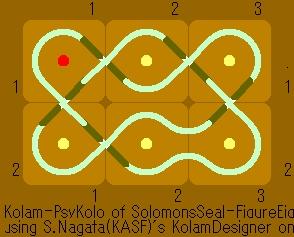
A kolam of a 2x3 dot array	The VISA Interlink Logo [1]	Version of the US bicentennial emblem
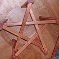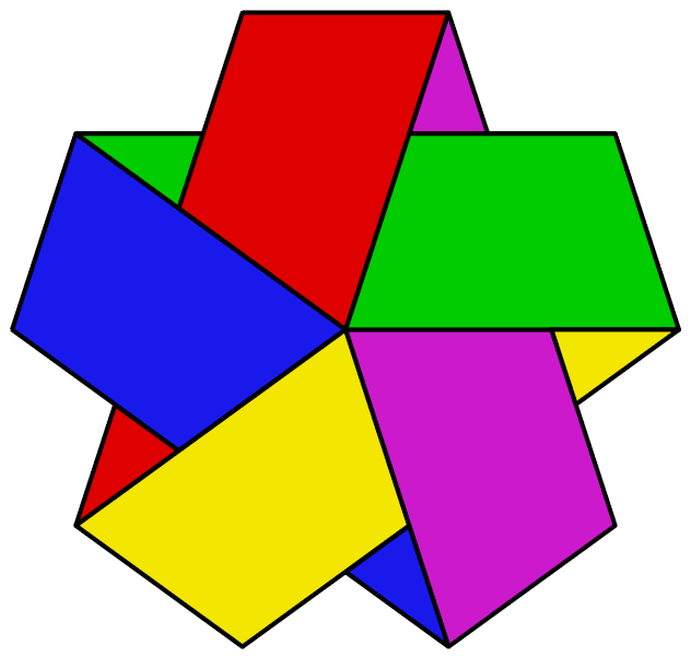
A pentagonal table by Bob Mackay [2]	The Utah State Parks logo	As impossible object ("Penrose" pentagram)
Folded ribbon which is single-sided (more complex version of Möbius Strip).	Non-pentagonal shape.	Pentagram of circles.
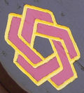
Alternate pentagram of intersecting circles.	3D-looking rendition.	Partial view of US bicentennial logo on a shirt seen in Lisboa [3]
Non-prime knot with two 5_1 configurations on a closed loop.	Knotted epitrochoid	Sum of two 5_1s, Vienna, orthodox church

This sentence was last edited by Dror. Sometime later, Scott added this sentence.

Knot presentations

Planar diagram presentation	X1627 X3849 X5,10,6,1 X7283 X9,4,10,5
Gauss code	-1, 4, -2, 5, -3, 1, -4, 2, -5, 3
Dowker-Thistlethwaite code	6 8 10 2 4
Conway Notation	[5]

Three dimensional invariants

Symmetry type Reversible Unknotting number 2 3-genus 2 Bridge index 2 Super bridge index 3 Nakanishi index 1 Maximal Thurston-Bennequin number [-10][3] Hyperbolic Volume Not hyperbolic A-Polynomial See Data:5 1/A-polynomial

[edit Notes for 5 1's three dimensional invariants]

Four dimensional invariants

Smooth 4 genus $2$ Topological 4 genus $2$ Concordance genus ${\textrm {ConcordanceGenus}}({\textrm {Knot}}(5,1))$ Rasmussen s-Invariant -4

[edit Notes for 5 1's four dimensional invariants]

Polynomial invariants

Alexander polynomial	$t^{2}+t^{-2}-t-t^{-1}+1$
Conway polynomial	$z^{4}+3z^{2}+1$
2nd Alexander ideal (db, data sources)	$\{1\}$
Determinant and Signature	{ 5, -4 }
Jones polynomial	$-q^{-7}+q^{-6}-q^{-5}+q^{-4}+q^{-2}$
HOMFLY-PT polynomial (db, data sources)	$a^{6}\left(-z^{2}\right)-2a^{6}+a^{4}z^{4}+4a^{4}z^{2}+3a^{4}$
Kauffman polynomial (db, data sources)	$a^{9}z+a^{8}z^{2}+a^{7}z^{3}-a^{7}z+a^{6}z^{4}-3a^{6}z^{2}+2a^{6}+a^{5}z^{3}-2a^{5}z+a^{4}z^{4}-4a^{4}z^{2}+3a^{4}$
The A2 invariant	$-q^{22}-q^{20}-q^{18}+q^{14}+q^{12}+2q^{10}+q^{8}+q^{6}$
The G2 invariant	$q^{120}-q^{100}-q^{98}-q^{92}-q^{90}-q^{88}-q^{82}-q^{80}-q^{78}-q^{72}+q^{58}+q^{56}+q^{52}+2q^{50}+q^{48}+q^{46}+q^{44}+q^{42}+2q^{40}+q^{38}+q^{34}+q^{32}+q^{30}$

Further Quantum Invariants

Further quantum knot invariants for 5_1.

A1 Invariants.

Weight	Invariant
1	$-q^{15}+q^{7}+q^{5}+q^{3}$
2	$q^{40}-q^{32}-q^{30}-q^{28}+q^{14}+q^{12}+q^{10}+q^{8}+q^{6}$
3	$-q^{75}+q^{67}+q^{65}+q^{63}-q^{49}-q^{47}-q^{45}-q^{43}-q^{41}+q^{21}+q^{19}+q^{17}+q^{15}+q^{13}+q^{11}+q^{9}$
4	$q^{120}-q^{112}-q^{110}-q^{108}+q^{94}+q^{92}+q^{90}+q^{88}+q^{86}-q^{66}-q^{64}-q^{62}-q^{60}-q^{58}-q^{56}-q^{54}+q^{28}+q^{26}+q^{24}+q^{22}+q^{20}+q^{18}+q^{16}+q^{14}+q^{12}$
5	$-q^{175}+q^{167}+q^{165}+q^{163}-q^{149}-q^{147}-q^{145}-q^{143}-q^{141}+q^{121}+q^{119}+q^{117}+q^{115}+q^{113}+q^{111}+q^{109}-q^{83}-q^{81}-q^{79}-q^{77}-q^{75}-q^{73}-q^{71}-q^{69}-q^{67}+q^{35}+q^{33}+q^{31}+q^{29}+q^{27}+q^{25}+q^{23}+q^{21}+q^{19}+q^{17}+q^{15}$
6	$q^{240}-q^{232}-q^{230}-q^{228}+q^{214}+q^{212}+q^{210}+q^{208}+q^{206}-q^{186}-q^{184}-q^{182}-q^{180}-q^{178}-q^{176}-q^{174}+q^{148}+q^{146}+q^{144}+q^{142}+q^{140}+q^{138}+q^{136}+q^{134}+q^{132}-q^{100}-q^{98}-q^{96}-q^{94}-q^{92}-q^{90}-q^{88}-q^{86}-q^{84}-q^{82}-q^{80}+q^{42}+q^{40}+q^{38}+q^{36}+q^{34}+q^{32}+q^{30}+q^{28}+q^{26}+q^{24}+q^{22}+q^{20}+q^{18}$
8	$q^{400}-q^{392}-q^{390}-q^{388}+q^{374}+q^{372}+q^{370}+q^{368}+q^{366}-q^{346}-q^{344}-q^{342}-q^{340}-q^{338}-q^{336}-q^{334}+q^{308}+q^{306}+q^{304}+q^{302}+q^{300}+q^{298}+q^{296}+q^{294}+q^{292}-q^{260}-q^{258}-q^{256}-q^{254}-q^{252}-q^{250}-q^{248}-q^{246}-q^{244}-q^{242}-q^{240}+q^{202}+q^{200}+q^{198}+q^{196}+q^{194}+q^{192}+q^{190}+q^{188}+q^{186}+q^{184}+q^{182}+q^{180}+q^{178}-q^{134}-q^{132}-q^{130}-q^{128}-q^{126}-q^{124}-q^{122}-q^{120}-q^{118}-q^{116}-q^{114}-q^{112}-q^{110}-q^{108}-q^{106}+q^{56}+q^{54}+q^{52}+q^{50}+q^{48}+q^{46}+q^{44}+q^{42}+q^{40}+q^{38}+q^{36}+q^{34}+q^{32}+q^{30}+q^{28}+q^{26}+q^{24}$

A2 Invariants.

Weight	Invariant
1,0	$-q^{22}-q^{20}-q^{18}+q^{14}+q^{12}+2q^{10}+q^{8}+q^{6}$
1,1	$q^{60}-2q^{36}-2q^{34}-4q^{32}-4q^{30}-3q^{28}+2q^{24}+4q^{22}+5q^{20}+4q^{18}+4q^{16}+2q^{14}+q^{12}$
2,0	$q^{54}+q^{52}+2q^{50}+q^{48}-2q^{44}-3q^{42}-3q^{40}-3q^{38}-2q^{36}-q^{34}+q^{28}+q^{26}+2q^{24}+2q^{22}+3q^{20}+2q^{18}+2q^{16}+q^{14}+q^{12}$
3,0	$-q^{96}-q^{94}-2q^{92}-2q^{90}-q^{88}+q^{86}+3q^{84}+4q^{82}+5q^{80}+4q^{78}+4q^{76}+2q^{74}+q^{72}-q^{70}-2q^{68}-3q^{66}-4q^{64}-5q^{62}-5q^{60}-5q^{58}-4q^{56}-3q^{54}-2q^{52}-q^{50}+q^{42}+q^{40}+2q^{38}+2q^{36}+3q^{34}+3q^{32}+4q^{30}+3q^{28}+3q^{26}+2q^{24}+2q^{22}+q^{20}+q^{18}$

A3 Invariants.

Weight	Invariant
0,1,0	$q^{50}-q^{36}-2q^{34}-3q^{32}-3q^{30}-2q^{28}-q^{26}+2q^{24}+3q^{22}+4q^{20}+3q^{18}+3q^{16}+q^{14}+q^{12}$
1,0,0	$-q^{29}-q^{27}-2q^{25}-q^{23}+q^{19}+2q^{17}+2q^{15}+2q^{13}+q^{11}+q^{9}$
1,0,1	$q^{80}+q^{58}+q^{56}+3q^{54}+3q^{52}+2q^{50}-q^{48}-5q^{46}-9q^{44}-12q^{42}-12q^{40}-9q^{38}-3q^{36}+2q^{34}+7q^{32}+10q^{30}+11q^{28}+10q^{26}+7q^{24}+5q^{22}+2q^{20}+q^{18}$

A4 Invariants.

Weight	Invariant
0,1,0,0	$q^{64}+q^{62}+q^{60}+q^{58}+q^{56}-q^{50}-2q^{48}-4q^{46}-5q^{44}-6q^{42}-6q^{40}-4q^{38}-q^{36}+2q^{34}+4q^{32}+7q^{30}+6q^{28}+6q^{26}+4q^{24}+3q^{22}+q^{20}+q^{18}$
1,0,0,0	$-q^{36}-q^{34}-2q^{32}-2q^{30}-q^{28}+q^{24}+2q^{22}+3q^{20}+2q^{18}+2q^{16}+q^{14}+q^{12}$

B2 Invariants.

Weight	Invariant
0,1	$-q^{50}-q^{36}-q^{32}-q^{30}+q^{26}+q^{22}+2q^{20}+q^{18}+q^{16}+q^{14}+q^{12}$
1,0	$q^{80}-q^{58}-q^{56}-q^{54}-q^{52}-2q^{50}-q^{48}-q^{46}-q^{44}+q^{38}+q^{36}+2q^{34}+q^{32}+2q^{30}+q^{28}+2q^{26}+q^{24}+q^{22}+q^{18}$

B3 Invariants.

Weight	Invariant
1,0,0	$q^{120}-q^{86}-q^{82}-q^{80}-2q^{78}-q^{76}-2q^{74}-q^{72}-2q^{70}-q^{68}-q^{66}-q^{64}+q^{58}+q^{56}+2q^{54}+q^{52}+3q^{50}+q^{48}+3q^{46}+q^{44}+2q^{42}+q^{40}+2q^{38}+q^{34}+q^{30}$

B4 Invariants.

Weight	Invariant
1,0,0,0	$q^{160}-q^{114}-q^{110}-2q^{106}-q^{104}-2q^{102}-q^{100}-2q^{98}-q^{96}-2q^{94}-q^{92}-2q^{90}-q^{88}-q^{86}+q^{78}+2q^{74}+q^{72}+3q^{70}+q^{68}+3q^{66}+q^{64}+3q^{62}+q^{60}+3q^{58}+q^{56}+2q^{54}+2q^{50}+q^{46}+q^{42}$

C3 Invariants.

Weight	Invariant
1,0,0	$-q^{70}-q^{50}-q^{48}-q^{46}-q^{44}-q^{42}-q^{40}+q^{34}+q^{32}+2q^{30}+2q^{28}+2q^{26}+q^{24}+2q^{22}+q^{20}+q^{18}$

C4 Invariants.

Weight	Invariant
1,0,0,0	$-q^{90}-q^{64}-q^{62}-2q^{60}-q^{58}-q^{56}-q^{54}-q^{52}-q^{50}-q^{48}+q^{44}+2q^{42}+2q^{40}+2q^{38}+2q^{36}+2q^{34}+2q^{32}+2q^{30}+2q^{28}+q^{26}+q^{24}$

D4 Invariants.

Weight	Invariant
0,1,0,0	$q^{120}-q^{100}-q^{98}-3q^{96}-3q^{94}-q^{92}-q^{90}+2q^{88}+6q^{86}+9q^{84}+11q^{82}+14q^{80}+11q^{78}+9q^{76}+3q^{74}-4q^{72}-12q^{70}-18q^{68}-24q^{66}-27q^{64}-27q^{62}-24q^{60}-17q^{58}-11q^{56}+7q^{52}+14q^{50}+19q^{48}+22q^{46}+19q^{44}+19q^{42}+14q^{40}+10q^{38}+6q^{36}+4q^{34}+q^{32}+q^{30}$
1,0,0,0	$q^{70}-q^{50}-q^{48}-3q^{46}-3q^{44}-3q^{42}-3q^{40}-2q^{38}+q^{34}+3q^{32}+4q^{30}+4q^{28}+4q^{26}+3q^{24}+2q^{22}+q^{20}+q^{18}$

G2 Invariants.

Weight	Invariant
0,1	$q^{240}-q^{198}-q^{192}+q^{178}+q^{176}+q^{172}+2q^{170}+q^{168}+q^{166}+q^{164}+q^{162}+2q^{160}+q^{158}+q^{154}+q^{152}-q^{148}-q^{146}-q^{144}-q^{142}-2q^{140}-3q^{138}-2q^{136}-2q^{134}-3q^{132}-4q^{130}-4q^{128}-3q^{126}-3q^{124}-4q^{122}-4q^{120}-3q^{118}-2q^{116}-2q^{114}-3q^{112}-2q^{110}+q^{102}+q^{100}+2q^{98}+3q^{96}+2q^{94}+2q^{92}+4q^{90}+3q^{88}+3q^{86}+4q^{84}+3q^{82}+3q^{80}+4q^{78}+2q^{76}+2q^{74}+3q^{72}+2q^{70}+q^{68}+2q^{66}+q^{64}+q^{62}+q^{60}+q^{54}$
1,0	$q^{120}-q^{100}-q^{98}-q^{92}-q^{90}-q^{88}-q^{82}-q^{80}-q^{78}-q^{72}+q^{58}+q^{56}+q^{52}+2q^{50}+q^{48}+q^{46}+q^{44}+q^{42}+2q^{40}+q^{38}+q^{34}+q^{32}+q^{30}$

.

Computer Talk

The above data is available with the Mathematica package KnotTheory`, as shown in the (simulated) Mathematica session below. Your input (in red) is realistic; all else should have the same content as in a real mathematica session, but with different formatting. This Mathematica session is also available (albeit only for the knot 5_2) as the notebook PolynomialInvariantsSession.nb.

(The path below may be different on your system, and possibly also the KnotTheory` date)

In[1]:=

AppendTo[$Path, "C:/drorbn/projects/KAtlas/"]; << KnotTheory`

Loading KnotTheory` version of August 31, 2006, 11:25:27.5625. Read more at http://katlas.math.toronto.edu/wiki/KnotTheory.

In[3]:=

K = Knot["5 1"];

In[4]:=

Alexander[K][t]

KnotTheory::loading: Loading precomputed data in PD4Knots`.

Out[4]=

$t^{2}+t^{-2}-t-t^{-1}+1$

In[5]:=

Conway[K][z]

Out[5]=

$z^{4}+3z^{2}+1$

In[6]:=

Alexander[K, 2][t]

KnotTheory::credits: The program Alexander[K, r] to compute Alexander ideals was written by Jana Archibald at the University of Toronto in the summer of 2005.

Out[6]=

$\{1\}$

In[7]:=

{KnotDet[K], KnotSignature[K]}

Out[7]=

{ 5, -4 }

In[8]:=

Jones[K][q]

KnotTheory::loading: Loading precomputed data in Jones4Knots`.

Out[8]=

$-q^{-7}+q^{-6}-q^{-5}+q^{-4}+q^{-2}$

In[9]:=

HOMFLYPT[K][a, z]

KnotTheory::credits: The HOMFLYPT program was written by Scott Morrison.

Out[9]=

$a^{6}\left(-z^{2}\right)-2a^{6}+a^{4}z^{4}+4a^{4}z^{2}+3a^{4}$

In[10]:=

Kauffman[K][a, z]

KnotTheory::loading: Loading precomputed data in Kauffman4Knots`.

Out[10]=

$a^{9}z+a^{8}z^{2}+a^{7}z^{3}-a^{7}z+a^{6}z^{4}-3a^{6}z^{2}+2a^{6}+a^{5}z^{3}-2a^{5}z+a^{4}z^{4}-4a^{4}z^{2}+3a^{4}$

Vassiliev invariants

V2 and V3:

(3, -5)

V2,1 through V6,9:

V2,1 V3,1 V4,1 V4,2 V4,3 V5,1 V5,2 V5,3 V5,4 V6,1 V6,2 V6,3 V6,4 V6,5 V6,6 V6,7 V6,8 V6,9 $12$ $-40$ $72$ $174$ $26$ $-480$ $-{\frac {2512}{3}}$ $-{\frac {448}{3}}$ $-104$ $288$ $800$ $2088$ $312$ ${\frac {41151}{10}}$ ${\frac {2494}{15}}$ ${\frac {7634}{5}}$ ${\frac {43}{2}}$ ${\frac {1951}{10}}$

V_2,1 through V_6,9 were provided by Petr Dunin-Barkowski <barkovs@itep.ru>, Andrey Smirnov <asmirnov@itep.ru>, and Alexei Sleptsov <sleptsov@itep.ru> and uploaded on October 2010 by User:Drorbn. Note that they are normalized differently than V₂ and V₃.

Khovanov Homology

The coefficients of the monomials $t^{r}q^{j}$ are shown, along with their alternating sums $\chi$ (fixed $j$, alternation over $r$). The squares with yellow highlighting are those on the "critical diagonals", where $j-2r=s+1$ or $j-2r=s-1$, where $s=$-4 is the signature of 5 1. Nonzero entries off the critical diagonals (if any exist) are highlighted in red.

\   r    \    j   \ -5 -4 -3 -2 -1 0 χ -3           1 1 -5           1 1 -7       1     1 -9             0 -11   1 1       0 -13             0 -15 1           -1

Integral Khovanov Homology (db, data source)

$\dim {\mathcal {G}}_{2r+i}\operatorname {KH} _{\mathbb {Z} }^{r}$ $i=-5$ $i=-3$ $r=-5$ ${\mathbb {Z} }$ $r=-4$ ${\mathbb {Z} }_{2}$ ${\mathbb {Z} }$ $r=-3$ ${\mathbb {Z} }$ $r=-2$ ${\mathbb {Z} }_{2}$ ${\mathbb {Z} }$ $r=-1$ $r=0$ ${\mathbb {Z} }$ ${\mathbb {Z} }$

Computer Talk

Much of the above data can be recomputed by Mathematica using the package KnotTheory`. See A Sample KnotTheory` Session.

${\textrm {Include}}({\textrm {ColouredJonesM.mhtml}})$

In[1]:=	<< KnotTheory`
Loading KnotTheory` (version of August 17, 2005, 14:44:34)...
In[2]:=	Crossings[Knot[5, 1]]
Out[2]=	5
In[3]:=	PD[Knot[5, 1]]
Out[3]=	PD[X[1, 6, 2, 7], X[3, 8, 4, 9], X[5, 10, 6, 1], X[7, 2, 8, 3], X[9, 4, 10, 5]]
In[4]:=	GaussCode[Knot[5, 1]]
Out[4]=	GaussCode[-1, 4, -2, 5, -3, 1, -4, 2, -5, 3]
In[5]:=	BR[Knot[5, 1]]
Out[5]=	BR[2, {-1, -1, -1, -1, -1}]
In[6]:=	alex = Alexander[Knot[5, 1]][t]
Out[6]=	-2 1 2 1 + t - - - t + t t
In[7]:=	Conway[Knot[5, 1]][z]
Out[7]=	2 4 1 + 3 z + z
In[8]:=	Select[AllKnots[], (alex === Alexander[#][t])&]
Out[8]=	{Knot[5, 1], Knot[10, 132]}
In[9]:=	{KnotDet[Knot[5, 1]], KnotSignature[Knot[5, 1]]}
Out[9]=	{5, -4}
In[10]:=	J=Jones[Knot[5, 1]][q]
Out[10]=	-7 -6 -5 -4 -2 -q + q - q + q + q
In[11]:=	Select[AllKnots[], (J === Jones[#][q] || (J /. q-> 1/q) === Jones[#][q])&]
Out[11]=	{Knot[5, 1], Knot[10, 132]}
In[12]:=	A2Invariant[Knot[5, 1]][q]
Out[12]=	-22 -20 -18 -14 -12 2 -8 -6 -q - q - q + q + q + --- + q + q 10 q
In[13]:=	Kauffman[Knot[5, 1]][a, z]
Out[13]=	4 6 5 7 9 4 2 6 2 8 2 3 a + 2 a - 2 a z - a z + a z - 4 a z - 3 a z + a z + 5 3 7 3 4 4 6 4 a z + a z + a z + a z
In[14]:=	{Vassiliev[2][Knot[5, 1]], Vassiliev[3][Knot[5, 1]]}
Out[14]=	{0, -5}
In[15]:=	Kh[Knot[5, 1]][q, t]
Out[15]=	-5 -3 1 1 1 1 q + q + ------ + ------ + ------ + ----- 15 5 11 4 11 3 7 2 q t q t q t q t