Printable Manual: Difference between revisions
No edit summary |
No edit summary |
||
| Line 1: | Line 1: | ||
<!-- don't edit independently of [[Manual TOC]]. See discussion page. --> |
<!-- don't edit independently of [[Manual TOC]]. See discussion page. --> |
||
{{Acknowledgement}} |
{{:Acknowledgement}} |
||
{{Setup}} |
{{:Setup}} |
||
{{Naming and Enumeration}} |
{{:Naming and Enumeration}} |
||
{{Presentations}} |
{{:Presentations}} |
||
{{Planar Diagrams]]}} |
{{:Planar Diagrams]]}} |
||
*** [[Planar Diagrams#Some further details|Some further details]] |
*** [[Planar Diagrams#Some further details|Some further details]] |
||
** [[Gauss Codes]] |
** [[Gauss Codes]] |
||
Revision as of 10:00, 29 August 2005
This Atlas is partially (and indirectly) supported by NSERC grant RGPIN 262178. As a Wiki project, it doesn't make sense anymore to acknowledge individual contributors. Yet for historical purposes, here's our acknowledgement as of the conversion to Wiki formnat on August 2005:
- Jana Archibald, for writing the program
Alexander[K, r]. - Sergei Chmutov, for spotting a typo.
- David De Wit, for a bug report.
- Ralph Furmaniak, for help with our link to Knotilus (see Gauss Codes).
- Stavros Garoufalidis, for jointly writing the program ColouredJones (see The Coloured Jones Polynomials).
- Thomas Gittings, for the minimum braid representatives for the knots with up to 10 crossings (see Braid Representatives).
- Jeremy Green, for his java implementation of
Kh(see Khovanov Homology). - Thang Le, for supplying some of the formulas used in the program ColouredJones (see The Coloured Jones Polynomials).
- Rick Litherland, for spotting a sneaky bug in the program
KnotSignature. - Charles Livingston, for allowing us to bundle data from his Table of Knot Invariants.
- Scott Morrison, for a bug report and for writing the programs to compute the HOMFLY-PT and Kauffman polynomials (see The HOMFLY-PT Polynomial and The Kauffman Polynomial).
- Bertrand Patureau-Mirand, for informing us of some mismatches in the link tables (now corrected).
- Jozef Przytycki, for correcting a typo.
- Stuart Rankin, for help with our link to Knotilus (see Gauss Codes).
- Emily Redelmeier, for writing the program DrawPD (see Drawing Planar Diagrams).
- Siddarth Sankaran, for writing the conversion program between Gauss codes and PD codes and for writing MorseLink and DrawMorseLink.
- Alexander Shumakovitch, for his help with signature computations (see The Determinant and the Signature).
- Alexander Stoimenow, for the knot presentations for the knots in the Rolfsen table and some further remarks.
- Z-X. Tao, for noticing problems with the knots 10_83 and 10_86.
- Morwen Thistlethwaite, for the pictures of links and of 11 crossing knots.
- Dylan Thurston, for writing an early routine to translate from Hoste-Thistlethwaite's DT codes to my "PD Presentations".
Start by downloading the file KnotTheory.zip (around 15MB), and unpack it. This will create a subdirectory KnotTheory/ in your current working directory. This done, no installation is required (though you may wish to check out Further Data Files and/or Setting the Path below). Start Mathematica and you're ready to go:
In[2]:= << KnotTheory`
Loading KnotTheory` version of March 22, 2011, 21:10:4.67737. Read more at http://katlas.org/wiki/KnotTheory.
Notice the little "prime" at the end of KnotTheory above. It is a backquote (find it on the upper left side of most keyboards) and not a quote, and it really has to be there for things to work.
Let us check that everything is working well:
In[3]:=
|
Alexander[Knot[6, 2]][t]
|
Out[3]=
|
      -2   3          2
-3 - t   + - + 3 t - t
           t
|
| ||||
| ||||
| ||||
Thus on the day this manual page was last changed, we had:
In[7]:=
|
{KnotTheoryVersion[], KnotTheoryVersionString[]}
|
Out[7]=
|
{{2011, 3, 22, 21, 10, 4.67737}, March 22, 2011, 21:10:4.67737}
|
In[8]:=
|
KnotTheoryWelcomeMessage[]
|
Out[8]=
|
Loading KnotTheory` version of March 22, 2011, 21:10:4.67737.
Read more at http://katlas.org/wiki/KnotTheory.
|
| ||||
In[10]:=
|
KnotTheoryDirectory[]
|
Out[10]=
|
C:\Documents and Settings\pc\Documenti\Wolfram\KnotTheory
|
KnotTheoryDirectory may not work under some operating systems/environments. Please let Dror know if you encounter any difficulties.
Notes
Precomputed Data
KnotTheory` comes with a certain amount of precomputed data which is loaded "on demand" just when it is needed. When a precomputed data file is read by KnotTheory`, a notification message is displayed. To prevent these messages from appearing execute the command Off[KnotTheory::loading].
Further Data Files
To access the Hoste-Thistlethwaite enumeration of knots with 12 to 16 crossings (see Naming and Enumeration), also download either the file DTCodes4Knots12To16.tar.gz or the file DTCodes4Knots12To16.zip (about 9MB each), and unpack either one into the directory KnotTheory/.
Setting the Path
The directions above are written on the assumption that the package KnotTheory` (more precisely, the directory KnotTheory/ containing the files that make this package), is somewhere on your Mathematica search path. Usually this will be the case if KnotTheory/ is a subdirectory of your current working directory. If for some reason Mathematica cannot find KnotTheory`, you may tell it where to look in either of the following three ways. Assume KnotTheory/ is a subdirectory of FullPathToKnotTheory:
- If you are using KnotTheory` rarely and you don't want to change system defaults, evaluate AppendTo[$Path,"FullPathToKnotTheory"] within Mathematica before attempting to load KnotTheory`.
- If you plan to use KnotTheory` often, you may want to move the directory KnotTheory/ into one of the directories on your path. Evaluate $Path within Mathematica to see what those are.
- Alternatively, you may permanently add FullPathToKnotTheory to your $Path. To do that, find your Mathematica base directory by evaluating $UserBaseDirectory (on Dror's laptop, this comes out to be C:\Users\Dror\AppData\Roaming\Mathematica), and then add the line AppendTo[$Path,"FullPathToKnotTheory/"] to the file $BaseDirectory/Kernel/init.m and restart Mathematica.
KnotTheory` comes loaded with some knot tables; currently, the Rolfsen table of prime knots with up to 10 crossings [Rolfsen], the Hoste-Thistlethwaite tables of prime knots with up to 16 crossings and the Thistlethwaite table of prime links with up to 11 crossings (see Knotscape):
(For In[1] see Setup)
| ||||
| ||||
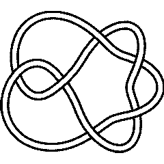 6_1 |
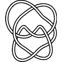 9_46 |
Thus, for example, let us verify that the knots 6_1 and 9_46 have the same Alexander polynomial:
In[4]:=
|
Alexander[Knot[6, 1]][t]
|
Out[4]=
|
    2
5 - - - 2 t
    t
|
In[5]:=
|
Alexander[Knot[9, 46]][t]
|
Out[5]=
|
    2
5 - - - 2 t
    t
|
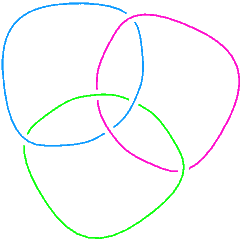 L6a4 |
We can also check that the Borromean rings, L6a4 in the Thistlethwaite table, is a 3-component link:
In[6]:=
|
Length[Skeleton[Link[6, Alternating, 4]]]
|
Out[6]=
|
3
|
| ||||
| ||||
Thus at the moment there are 1701936 knots and 5700 links known to KnotTheory`:
In[9]:=
|
Length /@ {AllKnots[{0,16}], AllLinks[{2,12}]}
|
Out[9]=
|
{1701936, 5700}
|
In[10]:=
|
Show[DrawPD[Knot[13, NonAlternating, 5016], {Gap -> 0.025}]]
|

| |
Out[10]=
|
-Graphics-
|
(Shumakovitch had noticed that this nice knot has interesting Khovanov homology; see [Shumakovitch]).
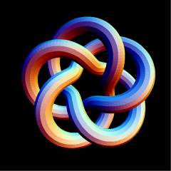 T(5,3) |
In addition to the tables, KnotTheory` also knows about torus knots:
| ||||
| ||||
For example, the torus knots T(5,3) and T(3,5) have different presentations with different numbers of crossings, but they are in fact isotopic, and hence they have the same invariants (and in particular the same type 3 Vassiliev invariant ):

In[13]:=
|
Crossings /@ {TorusKnot[5, 3], TorusKnot[3, 5]}
|
Out[13]=
|
{10, 12}
|
In[14]:=
|
Vassiliev[3] /@ {TorusKnot[5, 3], TorusKnot[3, 5]}
|
Out[14]=
|
{20, 20}
|
KnotTheory` knows how to plot torus knots; see Drawing with TubePlot.
You can also use the function Knot to parse certain string representations of named knots:
In[15]:=
|
Knot /@ {"K11a14", "11a_14", "L8a1", "T(3,5)"}
|
Out[15]=
|
{Knot[11, Alternating, 14], If[11 a <= 10 &&

    14 <= NumberOfKnots[11 a, Alternating] +

      NumberOfKnots[11 a, NonAlternating],

   Knot @@ KnotTheory`Naming`s$3008], Link[8, Alternating, 1],

  TorusKnot[3, 5]}
|
In the opposite direction, the function NameString produces the standard name for a knot, used throughout the Knot Atlas.
In[16]:=
|
NameString /@ {Knot[11, Alternating, 14], TorusKnot[3,5]}
|
Out[16]=
|
{K11a14, T(3,5)}
|
References
[Rolfsen] ^ D. Rolfsen, Knots and Links, Publish or Perish, Mathematics Lecture Series 7, Wilmington 1976.
[Shumakovitch] ^ A. Shumakovitch, Torsion of the Khovanov Homology, arXiv:math.GT/0405474.
KnotTheory` uses several presentations for knots/links.
- Planar Diagrams
- Gauss Codes
- DT (Dowker-Thistlethwaite) Codes
- Braid Representatives
- MorseLink Presentations
- Arc Presentations
- Conway Notation
{{:Planar Diagrams]]}}
- Graphical Output
- Structure and Operations
- Invariants
- Extras Included with KnotTheory`
- Lightly Documented Features
- Further Knot Theory Software
- How to Edit this Manual...
- About this Manual...
- Bibliography