Printable Manual

Download / Setup

This manual describes the Mathematica package KnotTheory`, the main tool used to produce The Knot Atlas.

Return to the wiki manual.

Acknowledgement

This Atlas is partially (and indirectly) supported by NSERC grant RGPIN 262178. As a Wiki project, it doesn't make sense anymore to acknowledge individual contributors. Yet for historical purposes, here's our acknowledgement as of the conversion to Wiki formnat on August 2005:

• Jana Archibald, for writing the program Alexander[K, r].
• Sergei Chmutov, for spotting a typo.
• David De Wit, for a bug report.
• Ralph Furmaniak, for help with our link to Knotilus (see Gauss Codes).
• Stavros Garoufalidis, for jointly writing the program ColouredJones (see The Coloured Jones Polynomials).
• Thomas Gittings, for the minimum braid representatives for the knots with up to 10 crossings (see Braid Representatives).
• Jeremy Green, for his java implementation of Kh (see Khovanov Homology).
• Thang Le, for supplying some of the formulas used in the program ColouredJones (see The Coloured Jones Polynomials).
• Rick Litherland, for spotting a sneaky bug in the program KnotSignature.
• Charles Livingston, for allowing us to bundle data from his Table of Knot Invariants.
• Scott Morrison, for a bug report and for writing the programs to compute the HOMFLY-PT and Kauffman polynomials (see The HOMFLY-PT Polynomial and The Kauffman Polynomial).
• Bertrand Patureau-Mirand, for informing us of some mismatches in the link tables (now corrected).
• Jozef Przytycki, for correcting a typo.
• Stuart Rankin, for help with our link to Knotilus (see Gauss Codes).
• Emily Redelmeier, for writing the program DrawPD (see Drawing Planar Diagrams).
• Siddarth Sankaran, for writing the conversion program between Gauss codes and PD codes and for writing MorseLink and DrawMorseLink.
• Alexander Shumakovitch, for his help with signature computations (see The Determinant and the Signature).
• Alexander Stoimenow, for the knot presentations for the knots in the Rolfsen table and some further remarks.
• Z-X. Tao, for noticing problems with the knots 10_83 and 10_86.
• Morwen Thistlethwaite, for the pictures of links and of 11 crossing knots.
• Dylan Thurston, for writing an early routine to translate from Hoste-Thistlethwaite's DT codes to my "PD Presentations".

Setup

Start by downloading either the file KnotTheory.tar.gz or the file KnotTheory.zip (around 3MB each), and unpack either one. This will create a subdirectory KnotTheory/ in your current working directory. This done, no installation is required (though you may wish to check out Further Data Files and/or Setting the Path below). Start Mathematica and you're ready to go:

In[2]:= << KnotTheory`

Loading KnotTheory` version of March 22, 2011, 21:10:4.67737. Read more at http://katlas.org/wiki/KnotTheory.

Notice the little "prime" at the end of KnotTheory above. It is a backquote (find it on the upper left side of most keyboards) and not a quote, and it really has to be there for things to work.

Let us check that everything is working well:

In[3]:=	Alexander[Knot[6, 2]][t]
Out[3]=	-2 3 2 -3 - t + - + 3 t - t t

In[4]:= ?KnotTheoryVersion KnotTheoryVersion[] returns the date of the current version of the package KnotTheory`. KnotTheoryVersion[k] returns the kth field in KnotTheoryVersion[].

In[5]:= ?KnotTheoryVersionString KnotTheoryVersionString[] returns a string containing the date and time of the current version of the package KnotTheory`. It is generated from KnotTheoryVersion[].

In[6]:= ?KnotTheoryWelcomeMessage KnotTheoryWelcomeMessage[] returns a string containing the welcome message printed when KnotTheory` is first loaded.

Thus on the day this manual page was last changed, we had:

In[7]:=	{KnotTheoryVersion[], KnotTheoryVersionString[]}
Out[7]=	{{2011, 3, 22, 21, 10, 4.67737}, March 22, 2011, 21:10:4.67737}

In[8]:=	KnotTheoryWelcomeMessage[]
Out[8]=	Loading KnotTheory` version of March 22, 2011, 21:10:4.67737. Read more at http://katlas.org/wiki/KnotTheory.

In[9]:= ?KnotTheoryDirectory KnotTheoryDirectory[] returns the best guess KnotTheory` has for its location on the host computer. It can be reset by the user.

In[10]:=	KnotTheoryDirectory[]
Out[10]=	C:\Documents and Settings\pc\Documenti\Wolfram\KnotTheory

KnotTheoryDirectory may not work under some operating systems/environments. Please let Dror know if you encounter any difficulties.

Notes

Precomputed Data

KnotTheory` comes with a certain amount of precomputed data which is loaded "on demand" just when it is needed. When a precomputed data file is read by KnotTheory`, a notification message is displayed. To prevent these messages from appearing execute the command Off[KnotTheory::loading].

Further Data Files

To access the Hoste-Thistlethwaite enumeration of knots with 12 to 16 crossings (see Naming and Enumeration), also download either the file DTCodes4Knots12To16.tar.gz or the file DTCodes4Knots12To16.zip (about 9MB each), and unpack either one into the directory KnotTheory/.

Setting the Path

The directions above are written on the assumption that the package KnotTheory` (more precisely, the directory KnotTheory/ containing the files that make this package), is somewhere on your Mathematica search path. Usually this will be the case if KnotTheory/ is a subdirectory of your current working directory. If for some reason Mathematica cannot find KnotTheory`, you may tell it where to look in either of the following three ways. Assume KnotTheory/ is a subdirectory of FullPathToKnotTheory:

1. If you are using KnotTheory` rarely and you don't want to change system defaults, evaluate AppendTo[$Path,"FullPathToKnotTheory"] within Mathematica before attempting to load KnotTheory`.
2. If you plan to use KnotTheory` often, you may want to move the directory KnotTheory/ into one of the directories on your path. Evaluate $Path within Mathematica to see what those are.
3. Alternatively, you may permanently add FullPathToKnotTheory to your $Path. To do that, find your Mathematica base directory by evaluating $UserBaseDirectory (on Dror's laptop, this comes out to be C:\Users\Dror\AppData\Roaming\Mathematica), and then add the line AppendTo[$Path,"FullPathToKnotTheory/"] to the file $BaseDirectory/Kernel/init.m and restart Mathematica.

Naming and Enumeration

KnotTheory` comes loaded with some knot tables; currently, the Rolfsen table of prime knots with up to 10 crossings [Rolfsen], the Hoste-Thistlethwaite tables of prime knots with up to 16 crossings and the Thistlethwaite table of prime links with up to 11 crossings (see Knotscape):

(For In[1] see Setup)

In[2]:= ?Knot Knot[n, k] denotes the kth knot with n crossings in the Rolfsen table. Knot[n, Alternating, k] (for n between 11 and 16) denotes the kth alternating n-crossing knot in the Hoste-Thistlethwaite table. Knot[n, NonAlternating, k] denotes the kth non alternating n-crossing knot in the Hoste-Thistlethwaite table.

In[3]:= ?Link Link[n, Alternating, k] denotes the kth alternating n-crossing link in the Thistlethwaite table. Link[n, NonAlternating, k] denotes the kth non alternating n-crossing link in the Thistlethwaite table.

6_1

9_46

Thus, for example, let us verify that the knots 6_1 and 9_46 have the same Alexander polynomial:

In[4]:=	Alexander[Knot[6, 1]][t]
Out[4]=	2 5 - - - 2 t t

In[5]:=	Alexander[Knot[9, 46]][t]
Out[5]=	2 5 - - - 2 t t

L6a4

We can also check that the Borromean rings, L6a4 in the Thistlethwaite table, is a 3-component link:

In[6]:=	Length[Skeleton[Link[6, Alternating, 4]]]
Out[6]=	3

In[7]:= ?AllKnots AllKnots[] return a list of all knots with up to 11 crossings. AllKnots[n_] returns a list of all knots with n crossings, up to 16. AllKnots[{n_, m_}] returns a list of all knots with between n and m crossings, and AllKnots[n_, Alternating|NonAlternating] returns all knots with n crossings of the specified type.

In[8]:= ?AllLinks AllLinks[] return a list of all links with up to 11 crossings. AllLinks[n_] returns a list of all links with n crossings, up to 12.

Thus at the moment there are 1701936 knots and 5700 links known to KnotTheory`:

In[9]:=	Length /@ {AllKnots[{0,16}], AllLinks[{2,12}]}
Out[9]=	{1701936, 5700}

In[10]:=	Show[DrawPD[Knot[13, NonAlternating, 5016], {Gap -> 0.025}]]
Out[10]=	-Graphics-

(Shumakovitch had noticed that this nice knot has interesting Khovanov homology; see [Shumakovitch]).

T(5,3)

In addition to the tables, KnotTheory` also knows about torus knots:

In[11]:= ?TorusKnot TorusKnot[m, n] represents the (m,n) torus knot.

In[12]:= ?TorusKnots TorusKnots[n_] returns a list of all torus knots with up to n crossings.

For example, the torus knots T(5,3) and T(3,5) have different presentations with different numbers of crossings, but they are in fact isotopic, and hence they have the same invariants (and in particular the same type 3 Vassiliev invariant $V_{3}$):

In[13]:=	Crossings /@ {TorusKnot[5, 3], TorusKnot[3, 5]}
Out[13]=	{10, 12}

In[14]:=	Vassiliev[3] /@ {TorusKnot[5, 3], TorusKnot[3, 5]}
Out[14]=	{20, 20}

KnotTheory` knows how to plot torus knots; see Drawing with TubePlot.

You can also use the function Knot to parse certain string representations of named knots:

In[15]:=	Knot /@ {"K11a14", "11a_14", "L8a1", "T(3,5)"}
Out[15]=	{Knot[11, Alternating, 14], If[11 a <= 10 && 14 <= NumberOfKnots[11 a, Alternating] + NumberOfKnots[11 a, NonAlternating], Knot @@ KnotTheory`Naming`s$3008], Link[8, Alternating, 1], TorusKnot[3, 5]}

In the opposite direction, the function NameString produces the standard name for a knot, used throughout the Knot Atlas.

In[16]:=	NameString /@ {Knot[11, Alternating, 14], TorusKnot[3,5]}
Out[16]=	{K11a14, T(3,5)}

References

[Rolfsen] ^  D. Rolfsen, Knots and Links, Publish or Perish, Mathematics Lecture Series 7, Wilmington 1976.

[Shumakovitch] ^  A. Shumakovitch, Torsion of the Khovanov Homology, arXiv:math.GT/0405474.

Presentations

KnotTheory` uses several presentations for knots/links.

• Planar Diagrams
  • Some further details
• Gauss Codes
• DT (Dowker-Thistlethwaite) Codes
• Braid Representatives
• MorseLink Presentations
• Arc Presentations
• Conway Notation

Planar Diagrams

The PD notation

In the "Planar Diagrams" (PD) presentation we present every knot or link diagram by labeling its edges (with natural numbers, 1,...,n, and with increasing labels as we go around each component) and by a list crossings presented as symbols $X_{ijkl}$ where $i$, $j$, $k$ and $l$ are the labels of the edges around that crossing, starting from the incoming lower edge and proceeding counterclockwise. Thus for example, the PD presentation of the knot above is:

$X_{1928}X_{3,10,4,11}X_{5362}X_{7,1,8,12}X_{9,4,10,5}X_{11,7,12,6}.$

(This of course is the Miller Institute knot, the mirror image of the knot 6_2)

(For In[1] see Setup)

In[2]:= ?PD PD[v1, v2, ...] represents a planar diagram whose vertices are v1, v2, .... PD also acts as a "type caster", so for example, PD[K] where K is a named knot (or link) returns the PD presentation of that knot.

In[3]:= PD::about The GaussCode to PD conversion was written by Siddarth Sankaran at the University of Toronto in the summer of 2005.

In[4]:= ?X X[i,j,k,l] represents a crossing between the edges labeled i, j, k and l starting from the incoming lower strand i and going counterclockwise through j, k and l. The (sometimes ambiguous) orientation of the upper strand is determined by the ordering of {j,l}.

Thus, for example, let us compute the determinant of the above knot:

In[5]:=

K = PD[ X[1,9,2,8], X[3,10,4,11], X[5,3,6,2], X[7,1,8,12], X[9,4,10,5], X[11,7,12,6] ];

In[6]:=	Alexander[K][-1]
Out[6]=	-11

Some further details

In[7]:= ?Xp Xp[i,j,k,l] represents a positive (right handed) crossing between the edges labeled i, j, k and l starting from the incoming lower strand i and going counter clockwise through j, k and l. The upper strand is therefore oriented from l to j regardless of the ordering of {j,l}. Presently Xp is only lightly supported.

In[8]:= ?Xm Xm[i,j,k,l] represents a negative (left handed) crossing between the edges labeled i, j, k and l starting from the incoming lower strand i and going counter clockwise through j, k and l. The upper strand is therefore oriented from j to l regardless of the ordering of {j,l}. Presently Xm is only lightly supported.

In[9]:= ?P P[i,j] represents a bivalent vertex whose adjacent edges are i and j (i.e., a "Point" between the segment i and the segment j). Presently P is only lightly supported.

For example, we could add an extra "point" on the Miller Institute knot, splitting edge 12 into two pieces, labeled 12 and 13:

In[10]:=

K1 = PD[ X[1,9,2,8], X[3,10,4,11], X[5,3,6,2], X[7,1,8,13], X[9,4,10,5], X[11,7,12,6], P[12,13] ];

At the moment, many of our routines do not know to ignore such "extra points". But some do:

In[11]:=	Jones[K][q] == Jones[K1][q]
Out[11]=	True

In[12]:= ?Loop Loop[i] represents a crossingsless loop labeled i.

Hence we can verify that the A2 invariant of the unknot is $q^{-2}+1+q^{2}$:

In[13]:=	A2Invariant[Loop[1]][q]
Out[13]=	-2 2 1 + q + q

Gauss Codes

The Gauss Code of an $n$-crossing knot or link $L$ is obtained as follows:

• Number the crossings of $L$ from 1 to $n$ in an arbitrary manner.
• Order the components of $L$ is some arbitrary manner.
• Start "walking" along the first component of $L$, taking note of the numbers of the crossings you've gone through. If in a given crossing you cross on the "over" strand, write down the number of that crossing. If you cross on the "under" strand, write down the negative of the number of that crossing.
• Do the same for all other components of $L$ (if any).

The resulting list of signed integers (in the case of a knot) or list of lists of signed integers (in the case of a link) is called the Gauss Code of $L$. KnotTheory` has some rudimentary support for Gauss codes:

(For In[1] see Setup)

In[2]:= ?GaussCode GaussCode[i1, i2, ...] represents a knot via its Gauss Code following the conventions used by the knotilus website, http://srankin.math.uwo.ca/cgi-bin/retrieve.cgi/html/start.html. Likewise GaussCode[l1, l2, ...] represents a link, where each of l1, l2,... is a list describing the code read along one component of the link. GaussCode also acts as a "type caster", so for example, GaussCode[K] where K is is a named knot (or link) returns the Gauss code of that knot.

Thus for example, the Gauss codes for the trefoil knot and the Borromean link are:

In[3]:=	GaussCode /@ {Knot[3, 1], Link[6, Alternating, 4]}
Out[3]=	{GaussCode[-1, 3, -2, 1, -3, 2], GaussCode[{1, -6, 5, -3}, {4, -1, 2, -5}, {6, -4, 3, -2}]}

3_1

L6a4

Ralph Furmaniak, working under the guidance of Stuart Rankin and Ortho Flint at the University of Western Ontario, wrote a web-based server called "Knotilus" that takes Gauss codes and outputs pictures of the desired knots and links in several standard image formats.

In[4]:= ?KnotilusURL KnotilusURL[K_] returns the URL of the knot/link K on the knotilus website, http://srankin.math.uwo.ca/cgi-bin/retrieve.cgi/html/start.html.

Thus,

In[5]:=	KnotilusURL /@ {Knot[3, 1], Link[6, Alternating, 4]}
Out[5]=	{http://srankin.math.uwo.ca/cgi-bin/retrieve.cgi/-1,3,-2,1,-3,2/goTop.h\ tml, http://srankin.math.uwo.ca/cgi-bin/retrieve.cgi/1,-6,5,-3:4,-1,\ 2,-5:6,-4,3,-2/goTop.html}

DT (Dowker-Thistlethwaite) Codes

Knots

The "DT Code" ("DT" after Clifford Hugh Dowker and Morwen Thistlethwaite) of a knot $K$ is obtained as follows:

• Start "walking" along $K$ and count every crossing you pass through. If $K$ has $n$ crossings and given that every crossing is visited twice, the count ends at $2n$. Label each crossing with the values of the counter when it is visited, though when labeling by an even number, take it with a minus sign if you are walking "over" the crossing.
• Every crossing is now labeled with two integers whose absolute values run from $1$ to $2n$. It is easy to see that each crossing is labeled with one odd integer and one even integer. The DT code of $K$ is the list of even integers paired with the odd integers 1, 3, 5, ..., taken in this order. Thus for example the pairing for the knot in the figure below is $((1,-8),(3,-10),(5,-2),(7,-12),(9,-4),(11,-6))$, and hence its DT code is $(-8,-10,-2,-12,-4,-6)$ (and as DT codes are insensitive to overall mirrors, this is equivalent to $(8,10,2,12,4,6)$).

The DT notation

KnotTheory` has some rudimentary support for DT codes:

(For In[1] see Setup)

In[2]:= ?DTCode DTCode[i1, i2, ...] represents a knot via its DT (Dowker-Thistlethwaite) code, while DTCode[{i11,...}, {i21...}, ...] likewise represents a link. DTCode also acts as a "type caster", so for example, DTCode[K] where K is is a named knot or link returns the DT code of K.

Thus for example, the DT codes for the last 9 crossing alternating knot 9_41 and the first 9 crossing non alternating knot 9_42 are:

In[3]:=	dts = DTCode /@ {Knot[9, 41], Knot[9, 42]}
Out[3]=	{DTCode[6, 10, 14, 12, 16, 2, 18, 4, 8], DTCode[4, 8, 10, -14, 2, -16, -18, -6, -12]}

(The DT code of an alternating knot is always a sequence of positive numbers but the DT code of a non alternating knot contains both signs.)

9_41

9_42

DT codes and Gauss codes carry the same information and are easily convertible:

In[4]:=	gcs = GaussCode /@ dts
Out[4]=	{GaussCode[1, -6, 2, -8, 3, -1, 4, -9, 5, -2, 6, -4, 7, -3, 8, -5, 9, -7], GaussCode[1, -5, 2, -1, 3, 8, -4, -2, 5, -3, -6, 9, -7, 4, -8, 6, -9, 7]}

In[5]:=	DTCode /@ gcs
Out[5]=	{DTCode[6, 10, 14, 12, 16, 2, 18, 4, 8], DTCode[4, 8, 10, -14, 2, -16, -18, -6, -12]}

Conversion between DT codes and/or Gauss codes and PD codes is more complicated; the harder side, going from DT/Gauss to PD, was written by Siddarth Sankaran at the University of Toronto:

In[6]:=	PD[DTCode[4, 6, 2]]
Out[6]=	PD[X[4, 2, 5, 1], X[6, 4, 1, 3], X[2, 6, 3, 5]]

Links

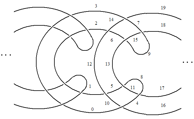
A DT notation example, for the link L7n2

DT Codes for links are defined in a similar way (see [DollHoste]). Follow the same numbering process as for knots, except when you finish traversing one component, jump straight to the next. It is not difficult to see that there is always a choice of starting points along the components for which the resulting pairing is a pairing between odd and even numbers. (On the figure above one possible choice is indicated). Again, it is enough to only list the even numbers corresponding to $1,3,5,\ldots$; call the resulting list $\lambda$. (Above, $\lambda =(6,-8,-10,12,-14,2,-4)$). Notice that the odd indices are naturally subdivided into sublists according to the component of the link on which they lie, and this induces a subdivision of $\lambda$ into sublists. Thus with the choices made in the figure above, the DT code for the link L7n2 is $(6,-8\mid -10,12,-14,2,-4)$.

KnotTheory` knows about DT codes for links:

In[7]:=	DTCode[Link[7, NonAlternating, 2]]
Out[7]=	DTCode[{6, -8}, {-10, 12, -14, 2, -4}]

In[8]:=	MultivariableAlexander[DTCode[{6, -8}, {-10, 12, -14, 2, -4}]][t]
Out[8]=	(-1 + t[1]) (-1 + t[2]) ----------------------- Sqrt[t[1]] Sqrt[t[2]]

[DollHoste] ^  H. Doll and J. Hoste, A tabulation of oriented links, Mathematics of Computation 57-196 (1991) 747-761.

Braid Representatives

Every knot and every link is the closure of a braid. KnotTheory` can also represent knots and links as braid closures:

(For In[1] see Setup)

In[2]:= ?BR BR stands for Braid Representative. BR[k, l] represents a braid on k strands with crossings l={i1, i2, ...}, where a positive index i within the list l indicates a right-handed crossing between strand number i and strand number i+1 and a negative i indicates a left handed crossing between strands numbers |i| and |i|+1. Each ij can also be a list of non-adjacent (i.e., commuting) indices. BR also acts as a "type caster": BR[K] will return a braid whose closure is K if K is given in any format that KnotTheory` understands. BR[K] where K is is a named knot with up to 10 crossings returns a minimum braid representative for that knot.

In[3]:= BR::about The minimum braids representing the knots with up to 10 crossings were provided by Thomas Gittings. See his article on the subject at arXiv:math.GT/0401051. Vogel's algorithm was implemented by Dan Carney in the summer of 2005 at the University of Toronto.

In[4]:= ?Mirror Mirror[br] return the mirror braid of br.

Thus for example,

In[5]:=

br1 = BR[2, {-1, -1, -1}];

In[6]:=	PD[br1]
Out[6]=	PD[X[6, 3, 1, 4], X[4, 1, 5, 2], X[2, 5, 3, 6]]

In[7]:=	Jones[br1][q]
Out[7]=	-4 -3 1 -q + q + - q

In[8]:=	Mirror[br1]
Out[8]=	BR[2, {1, 1, 1}]

T(5,4)

K11a362

KnotTheory` has the braid representatives of some knots and links pre-loaded, and for all other knots and links it will find a braid representative using Vogel's algorithm. Thus for example,

In[9]:=	BR[TorusKnot[5, 4]]
Out[9]=	BR[4, {1, 2, 3, 1, 2, 3, 1, 2, 3, 1, 2, 3, 1, 2, 3}]

In[10]:=	BR[Knot[11, Alternating, 362]]
Out[10]=	BR[10, {1, 2, -3, -4, 5, 6, 5, 4, 3, -2, -1, -4, 3, -2, -4, 3, 5, 4, -6, 7, -6, 5, 8, 7, 6, 5, -4, -3, 2, 5, -6, 9, -8, 7, -6, 5, 4, -3, 5, 6, 5, 4, 5, -7, 8, -7, 6, 5, -9, -8, -7}]

(As we see, Vogel's algorithm sometimes produces scary results. A 51-crossings braid representative for an 11-crossing knot, in the case of K11a362).

10_1

5_2

The minimum braid representative of a given knot is a braid representative for that knot which has a minimal number of braid crossings and within those braid representatives with a minimal number of braid crossings, it has a minimal number of strands (full details are in [Gittings]). Thomas Gittings kindly provided us the minimum braid representatives for all knots with up to 10 crossings. Thus for example, the minimum braid representative for the knot 10_1 has length (number of crossings) 13 and width 6 (number of strands, also see Invariants from Braid Theory):

In[11]:=	br2 = BR[Knot[10, 1]]
Out[11]=	BR[6, {-1, -1, -2, 1, -2, -3, 2, -3, -4, 3, 5, -4, 5}]

In[12]:=	Show[BraidPlot[CollapseBraid[br2]]]
Out[12]=	-Graphics-

Already for the knot 5_2 the minimum braid is shorter than the braid produced by Vogel's algorithm. Indeed, the minimum braid is

In[13]:=	Show[BraidPlot[CollapseBraid[BR[Knot[5, 2]]]]]
Out[13]=	-Graphics-

To force KnotTheory` to run Vogel's algorithm on 5_2, we first convert it to its PD form,

In[14]:=	pd = PD[Knot[5, 2]]
Out[14]=	PD[X[1, 4, 2, 5], X[3, 8, 4, 9], X[5, 10, 6, 1], X[9, 6, 10, 7], X[7, 2, 8, 3]]

and only then run BR:

In[15]:=	Show[BraidPlot[CollapseBraid[BR[pd]]]]
Out[15]=	-Graphics-

(Check Drawing Braids for information about the command BraidPlot and the related command CollapseBraid.)

[Gittings] ^  T. A. Gittings, Minimum braids: a complete invariant of knots and links, arXiv:math.GT/0401051.

MorseLink Presentations

The MorseLink presentation describes an oriented knot or link diagram as a sequence of 'events'. To begin, we fix an axis in the plane, so that each event in the MorseLink description occurs in successive intervals along this axis. The 'events' that comprise a knot or link are 'cups' (creations), 'caps' (annihilations), and crossings, where cups and caps are the minima and maxima (respectively) relative to the chosen axis. The conventions used by MorseLink are as follows:

• Cup[m,n] represents a creation, where the new strands are in position m and n, with m and n differing by 1, and is directed from m to n.
• Cap[m,n] represents an annihilation of the strands m and n, again with m and n differing by 1, and is directed from m to n.
• X[n, d, a, b] is a crossing of the n-th and the (n+1)-th strands. 'd' signifies whether the n-th strand goes 'Over' or 'Under' the (n+1)-th strand. 'a' indicates whether the n-th strand is moving 'Up' or 'Down' through the crossing, relative to the chosen axis; 'b' does the same for the (n+1)-th strand.

For concreteness, let us find a MorseLink presentation of the knot 4_1, based on the following diagram:

A diagram of the knot 4_1

We fix the chosen axis to be the positive $x$ axis, and we number the strands at each interval from bottom to top. Clearly the first event to take place is a cup, creating strands 1 and 2, and directed from 1 to 2. The next event is also a cup; this time, the strands 3 and 4 are created, from 3 to 4. So the first two elements of our MorseLink presentation are {Cup[1,2], Cup[3,4], ...}.

The next event to take place is a crossing. This crossing has strand 2 going under strand 3; following the orientations, strand 2 moves to the right through the crossing, while strand 3 comes from the left. Since the chosen axis is pointing to the right, this event is described as X[2, Under, Up, Down]. We may proceed in a similar way for the rest of the crossings.

After three more crossings, we encounter two cap events. The first annihilates strands 2 and 3, and is directed from 2 to 3. The second annihilates strands 1 and 2, but is directed from 2 to 1. So the MorseLink presentation for the knot 4_1 is given by: MorseLink[Cup[1,2], Cup[3,4], X[2 , Under, Up, Down], X[2, Under, Down, Up], X[1, Over, Down, Up], X[1, Over, Up, Down], Cap[2,3], Cap[2,1]].

Further notes

KnotTheory` knows about Morse link presentations: (For In[1] see Setup)

In[2]:= ?MorseLink MorseLink[K] returns a presentation of the oriented link K, composed, in successive order, of the following 'events': Cup[m,n] is a directed creation, starting at strand position n, towards position m, where m and n differ by 1. X[n,a = {Over/Under}, b = {Up/Down}, c={Up/Down}] is a crossing with lower-left edge at strand n, a determines whether the strand running bottom-left to top-right is over/under the crossing, b and c give the directions of the bottom-left and bottom-right strands respectively through the crossing. Cap[m,n] is a directed cap, from strand m to strand n.

In[3]:= MorseLink::about MorseLink was added to KnotTheory` by Siddarth Sankaran at the University of Toronto in the summer of 2005.

• Obviously, there is no unique Morse link presentation for a knot. One presentation may be considered 'better' than another if it generally has fewer strands. Unfortunately, this program makes only a half-hearted attempt in coming up with such presentations; it does a creation only when it can no longer do any caps or crossings, but exhibits a lack of foresight into which edges to create.

Arc Presentations

An Arc Presentation $A$ of a knot $K$ (in "grid form", to be precise) is a planar (toroidal, to be precise) picture of the knot in which all arcs are either horizontal or vertical, in which the vertical arcs are always "above" the horizontal arcs, and in which no two horizontal arcs have the same $y$-coordinate and no two vertical arcs have the same $x$-coordinate (read more at [1]). Without loss of generality, the $x$-coordinates of the vertical arcs in $A$ are the integers $1$ through $n$ for some $n$, and the $y$-coordinates of the horizontal arcs in $A$ are (also!) the integers $1$ through $n$.

((5,2), (1,3), (2,4), (3,5), (4,1))

Thus for example, on the left is an arc presentation $A$ of the trefoil knot. It can be represented numerically by the sequence of ordered pairs shown below it. This sequence reads: the lowest horizontal arc in $A$ connects the 5th vertical arc with the 2nd; the next horizontal arc in $A$ connects the 1st vertical with the 3rd, and so on. In general, an arc presentation involving $n$ horizontal and $n$ vertical arcs will be described in this way by a sequence of $n$ ordered pairs of integers in the range between $1$ and $n$.

Arc presentations are used extensively in the computation of Heegaard Floer Knot Homologies.

KnotTheory` knows about arc presentations:

(For In[1] see Setup)

In[1]:= ?ArcPresentation ArcPresentation[{a1,b1}, {a2, b2}, ..., {an,bn}] is an arc presentation of a knot (as often used in the realm of Heegaard-Floer homologies), where the horizontal arc at row i connects column ai to column bi. ArcPresentation[K] returns an arc presentation of the knot K. ArcPresentation[K, Reduce -> r] attemps at most r reduction steps (using a naive reduction algorithm) following a naive creation of some arc presentation for K.

K11n11

In[2]:=	ap = ArcPresentation["K11n11"]
Out[2]=	ArcPresentation[{12, 2}, {1, 10}, {3, 9}, {5, 11}, {9, 12}, {4, 8}, {2, 5}, {11, 7}, {8, 6}, {7, 4}, {10, 3}, {6, 1}]

In[4]:=	Draw[ap]
Out[4]=	-Graphics-

In[5]:=	ap0 = ArcPresentation["K11n11", Reduce -> 0]
Out[5]=	ArcPresentation[{13, 19}, {20, 23}, {19, 22}, {15, 14}, {14, 2}, {1, 13}, {3, 12}, {2, 4}, {16, 18}, {17, 15}, {8, 16}, {12, 17}, {5, 7}, {4, 6}, {7, 11}, {6, 8}, {18, 10}, {11, 9}, {10, 21}, {9, 20}, {21, 5}, {22, 3}, {23, 1}]

In[6]:= ?Draw Draw[ap] draws the Arc Presentation ap. Draw[ap, OverlayMatrix -> M] overlays the matrix M on top of that draw.

In[8]:=	Draw[ap0]
Out[8]=	-Graphics-

In[9]:=

Reflect[ap_ArcPresentation] := ArcPresentation @@ ( (Last /@ Sort[Reverse /@ Position[ap, #]]) & /@ Range[Length[ap]] )

In[11]:=	Reflect[ap] // Draw
Out[11]=	-Graphics-

The Minesweeper Matrix $M_{A}$ (name not generally accepted) of an arc presentation $A$ of $n$ rows/columns is the $n\times n$ matrix whose $(ij)$ entry is the rotation number of $A$ around a point placed between the $i$ and $i+1$ rows of $A$ and between the $j$ and $j+1$ column of $A$. Here's a little program to compute the minesweeper matrix of a given arc presentation, along with its output on the arc presentation of K11n11 that we have been studying above:

In[12]:=

MinesweeperMatrix[ap_ArcPresentation] := Module[ {l, CurrentRow, c1, c2, k, s}, l = Length[ap]; CurrentRow = Table[0, {l}]; Table[ {c1, c2} = Sort[ap[[k]]]; s = Sign[{-1, 1}.ap[[k]]]; Do[ CurrentRow[[c]] += s, {c, c1, c2 - 1} ]; CurrentRow, {k, l} ] ];

In[14]:=	Draw[ap, OverlayMatrix -> MinesweeperMatrix[ap]]
Out[14]=	-Graphics-

If $M_{A}=(m_{ij})$, it is known that the determinant of the matrix $(t^{m_{ij}})$ is the Alexander polynomial of the knot presented by $A$, up to signs and powers of $t$ and $(t-1)$. Let us check this in our case:

In[15]:=	{Det[t^MinesweeperMatrix[ap]], Alexander[ap][t]} // Factor
Out[15]=	11 2 2 3 4 5 6 {(-1 + t) t (1 - 5 t + 13 t - 17 t + 13 t - 5 t + t ), 2 3 4 5 6 1 - 5 t + 13 t - 17 t + 13 t - 5 t + t -------------------------------------------} 3 t

Conway Notation

Conway notation and KnotTheory`

KnotTheory` understands the Conway notation for knots and links (see [Conway] and down below), although the conversion between Conway notation and other knot presentations known to KnotTheory` (a necessary first step for using most of the KnotTheory` functionality) requires the packages K2K (KNOT 2000, by M.Ochiai and N.Imafuji) and LinKnot (by S. Jablan and R. Sazdanovic). For the download and installation of the LinKnot package see Using the LinKnot package.

(For In[1] see Setup)

As in the section Using the LinKnot package, the first step is to add LinKnot to the Mathematica search path. This path will likely be different on your computer. (Note that you can also use Conway notations in KnotTheory` if you are using KnotTheory` and LinKnot "in parallel", as described in Using the LinKnot package.)

In[2]:=

AppendTo[$Path, "C:/bin/LinKnot/"];

In[3]:= ?ConwayNotation ConwayNotation[s] represents the knot or link whose Conway notation is the string s. ConwayNotation[K], where K is a knot or a link with up to 12 crossings, returns ConwayNotation[s], where s is a string containing the Conway notation of K.

In[4]:= ConwayNotation::about The program ConwayNotation relies on code from the LinKnot package by Slavik Jablan and Ramila Sazdanovic.

A well known example of a knot with an Alexander polynomial equal to the Alexander polynomial of the unknot is the (-3,5,7)-pretzel knot $K$. Let us verify that, check (using the Jones polynomial) that $K$ is not the unknot and find a (rather unattractive) braid whose closure is $K$:

In[6]:=	DrawMorseLink[K = ConwayNotation["-3,5,7"]] // Show
Out[6]=	-Graphics-

In[7]:=	Alexander[K][t]
Out[7]=	1

In[8]:=	Jones[K][q]
Out[8]=	-12 -11 -10 2 -8 -7 -5 -4 2 -2 1 q - q + q - -- + q - q + q - q + -- - q + - 9 3 q q q

In[9]:=	br = BR[K]
Out[9]=	BR[14, {1, 2, 3, -4, -5, -6, -7, 8, -7, 6, 5, 4, -3, -2, -1, -6, -5, -4, -3, -2, 9, 8, 7, 6, -5, 4, -3, 7, -8, -7, -9, -8, 10, 9, -8, -11, -10, 12, 11, -10, 9, -8, -13, -12, -11, 10, 9, -8, -7, 6, -5, 4, -5, -7, 8, -7, -6, -7, -9, 8, -7, 6, 5, -4, 3, 2, -6, -7, -10, -9, 11, 10, -9, 8, -7, 6, 5, -4, 3, -6, 5, 4, -6, 5, 7, 6, -7, -8, 9, 8, -7, 12, -11, 10, -9, 13, -12, 11, -10}]

In[11]:=	BraidPlot[br] // Show
Out[11]=	-Graphics-

Some generalities about the Conway notation

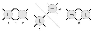
Conway notation was introduced by J.H. Conway in 1967 (see [Conway]). The main building blocks for Conway notation are 4-tangles. A 4-tangle in a knot or link projection is a region in the projection plane ${\mathbb {R} }^{2}$ (or on the sphere $S^{3}$) surrounded with a circle such that the projection intersects with the circle exactly four times. The elementary tangles are:

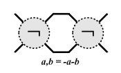
Tangles can be combined and modified by a unary operation $a\mapsto -a$ and three binary operations: sum, product and ramification, taking tangles $a$, $b$ to new tangles $a+b$, $a\,b$ and $a,b$. Here $-a$ is the image of $a$ under reflection in the NW-SE mirror line, $a+b$ is obtained by placing $a$ and $b$ side by side with $a$ on the left and $b$ on the right. $a\,b$ is simply $(-a)+b$, and finally, $a,b=(-a)+(-b)$.

Sum and product of tangles	Ramification of tangles

A rational tangle is any tangle obtained from the elementary tangles using only the operation of product. A rational knot or a rational link is the numerator closure of a rational tangle. A knot or link is called algebraic if it can be obtained as the closure of a tangle obtained from rational tangles using the operations above.

Knot or links that can not be obtained in this way are called non-algebraic. They can all be obtained in the following manner: start with a basic polyhedron $P$, a 4-valent graph without digons, with vertices numbered $1$ through $n$. Now substitute tangles $t_{1}$ through $t_{n}$ into these vertices.

The Conway notation for such knots and links consists of the symbol $ni^{\star }$ of a basic polyhedron $P$ where $n$ is the number of vertices and $i$ is the index of $P$ in some fixed list of basic polyhedra with $n$ vertices, followed by the symbols for the tangles $t_{1}$ through $t_{n}$ separated by dots.

For example, the knot 4_1 is denoted by "2 2", the knot 9_5 by "5 1 3", the link L5a1 is denoted by "2 1 2", the link L9a24 by "3 1,3,2" (all of them contain spaces between tangles), etc. A sequence of k pluses at the end of Conway symbol is denoted by +k, and the sequence of k minuses by +-k (e.g., knot 10_76 given in Conway notation as 3,3,2++ is denoted by "3,3,2+2", and the mirror of the link L9n21 whose Conway notation is 3,2,2,2-- is given by "3,2,2,2+-2"). The space is used in the same way in all other symbols.

For the basic polyhedra with $N<10$ crossings the standard notation is used (.1 , 6*, 8*, 9*, where the symbol for 6* can be ommitted). For example, the knot 10_95 is denoted by ".2 1 0.2.2", and 10_101 by "2 1..2..2". For higher values of $N$ a notation is used in which the first number is the number of crossings, and the next is the ordering number of polyhedron (e.g., 101*, 102*, 103* for $N=10$ denoting 10*, 10**, 10***, respectively, and 111*, 112*, 113* for $N=11$ denoting 11*, 11**, 11***, respectively, etc.).

The order of basic polyhedra for $N=12$ corresponds to the list in [Caudron], so 121* to 1212* denote the basic polyhedra originally titled as 12A-12L. For $N>12$ the database of basic polyhedra is produced from the list of simple 4-regular 4-edge-connected but not 3-connected plane graphs generated by Brendan McKay using the program "plantri" written by Gunnar Brinkmann and Brendan McKay (http://cs.anu.edu.au/~bdm/plantri/). PolyBase.m is automatically downloaded and it contains basic polyhedra up to 16 crossings. In order to work with the basic polyhedra up to 20 vertices, one needs to open an additional database PolyBaseN.m, for $N=17$ to $N=20$ (by writing, e.g. <<PolyBase17.m or Needs["PolyBase17.m"] for $N=17$).

Note: Together with the classical notation, Conway symbols are given in the book Knots and Links by D.~Rolfsen. However if you try to draw some knots or links from their Conway symbols the obtained projection might be non-isomorphic with the one given in Rolfsen, for example knot 9_15 denoted in Conway notation as 2 3 2 2 gives projection with 5, and not 4 digons.

[Caudron] ^  A. Caudron, Classification des noeuds et des enlancements. Public. Math. d'Orsay 82. Orsay: Univ. Paris Sud, Dept. Math., 1982.

[Conway] ^  J. H. Conway, An Enumeration of Knots and Links, and Some of Their Algebraic Properties. In Computation Problems in Abstract Algebra (Ed. J. Leech). Oxford, England: Pergamon Press, pp. 329-358, 1967.

Graphical Input

Thanks to our link with LinKnot, on Windows systems KnotTheory` accepts graphical knot input.

(For In[1] see Setup)

As in the section Using the LinKnot package, the first step is to add LinKnot to the Mathematica search path. This path will likely be different on your computer.

In[2]:=

AppendTo[$Path, "C:/bin/LinKnot/"];

In[3]:= ?KnotInput KnotInput[] opens a window in which you can draw a knot or link by hand. Right click and select 'Quit' when you're done. This function requires the package LinKnots`, and will only run on Windows machines. Sorry!

In[4]:= KnotInput::about The KnotInput program was written by M. Ochiai, C. Nakai, Y. Matsuyama and N. Imafuji and is imported to KnotTheory` via the package LinKnot by S. Jablan and R. Sazdanovic

Thus for example, the input line

In[5]:=

K = KnotInput[]

pops a blank window on which a knot or a link can be drawn with mouse clicks. At first pass all crossings are drawn as "new over old", but a further click on any given crossing will flip it.

KnotInput in action.

A right click followed by selecting "quit" will then determine the Gauss code of the knot or link just drawn and return it to Mathematica:

Out[5]=

GaussCode[{-1,-4,2,3},{-3,-5,4,6},{5,1,-6,-2}]

K is now perfectly usable within KnotTheory`:

In[5]:=	Kh[K][q, t]
Out[5]=	3 5 7 2 11 3 9 4 11 4 13 4 q + q + q t + q t + q t + 3 q t + 2 q t

Graphical Output

KnotTheory` can draw knots and links in several ways.

Drawing Planar Diagrams

My summer student Emily Redelmeier is in the process of writing a program that uses circle packing to draw an arbitrary object given as a PD as in Planar Diagrams. At the moment her program is still slow, limited and sometimes buggy, but it is already quite useful, as the following lines show:

(For In[1] see Setup)

In[2]:= ?DrawPD DrawPD[pd] takes the planar diagram description pd and creates a graphics object containing a picture of the knot. DrawPD[pd,options], where options is a list of rules, allows the user to control some of the parameters. OuterFace->n sets the face at infinity to the face numbered n. OuterFace->{e_1,e_2,...,e_n} sets the face at infinity to a face which has edges e_1, e_2, ..., e_n in the planar diagram description. Gap->g sets the size of the gap around a crossing to length g.

In[3]:= DrawPD::about DrawPD was written by Emily Redelmeier at the University of Toronto in the summers of 2003 and 2004.

Thus, for example, here's the torus knot T(4,3):

In[4]:=	Show[DrawPD[TorusKnot[4, 3]]]
Out[4]=	-Graphics-

One problem we currently have is that crossings come out at non-uniform sizes, hence in the picture below you may need magnifying glasses to decide who's over and who's under:

In[5]:=

MillettUnknot = PD[ X[1,10,2,11], X[9,2,10,3], X[3,7,4,6], X[15,5,16,4], X[5,17,6,16],X[7,14,8,15], X[8,18,9,17], X[11,18,12,19], X[19,12,20,13], X[13,20,14,1] ];

In[6]:=	Show[DrawPD[MillettUnknot]]
Out[6]=	-Graphics-

In such a situation, the option Gap is sometimes handy:

In[7]:=	Show[DrawPD[MillettUnknot, {Gap -> 0.03}]]
Out[7]=	-Graphics-

How does it work?

DrawPD uses Andreev's theorem [Andreev1], [Andreev2], which states that every planar graph can be realized, nearly uniquely, as the graph of tangencies of circles drawn within the unit disk. That is, to every vertex of $G$ one may associate a disk within the unit disk, so that the interiors of these disks are disjoint and they are tangent iff the corresponding vertices are connected by an edge. The Andreev "circle packing" corresponding to the knot 4_1 is the first picture on the right (circle 13 is the unit disk itself).

But now every ingredient of the original knot (every arc, crossing and face) has a disk in the plane in which it can be cleanly drawn and clashes are guaranteed not to occur. Furthermore, knowing the precise coordinates of all the tangency points allows us to represent each ingredient by some nice smooth arcs that meet smoothly. The result is the second picture on the right. Removing all the circles, what remains is the desired clean planar picture of 4_1.

[Andreev1] ^  A. Andreev, On convex polyhedra in Lobacevskii spaces (in Russian), Math. Sbornik USSR, Nov. Ser. 81 (1970) 445-478.

[Andreev2] ^  A. Andreev, On convex polyhedra of finite volume in Lobacevskii spaces (in Russian), Math. Sbornik USSR, Nov. Ser. 83 (1970) 256-260.

Drawing MorseLink Presentations

KnotTheory` can also draw knots and links via their Morse link presentations:

(For In[1] see Setup)

In[1]:= ?DrawMorseLink DrawMorseLink[L] returns a drawing of the knot or link L as a "Morse Link". For diagrams with a large number of crossings, it may be helpful to use one or both of the options as in DrawMorseLink[L, Gap -> g, ArrowSize -> as ], with 0 < as, g < 1, where g controls the amount of white space at each crossing, and as controls the size of the orientation arrows.

In[2]:= DrawMorseLink::about DrawMorseLink was written by Siddarth Sankaran at the University of Toronto in the summer of 2005.

For example, here is the 11-crossing alternating link L11a548:

In[4]:=	Show[DrawMorseLink[Link[11, Alternating, 548]]]
Out[4]=	-Graphics-

There are two options available for this program. Adding the option Gap -> g, where g is between 0 and 1, changes the amount of white space in each crossing; increasing g increases the white space, making large diagrams more visible. The option ArrowSize -> as (where as is between 0 and 1) alters the size of the orientation arrows. Here is the same drawing as above, but this time the orientation arrows are gone and the crossings are more clear:

In[6]:=	Show[DrawMorseLink[ Link[11, Alternating, 548], ArrowSize -> 0, Gap -> 0.65 ]]
Out[6]=	-Graphics-

Drawing Braids

(For In[1] see Setup)

In[2]:= ?BraidPlot BraidPlot[br, opts] produces a plot of the braid br. Possible options are Mode, HTMLOpts, WikiOpts and Images.

Thus for example,

In[3]:=

br = BR[5, {{1,3}, {-2,-4}, {1, 3}}];

In[4]:=	Show[BraidPlot[br]]
Out[4]=	-Graphics-

BraidPlot takes several options:

In[5]:=	Options[BraidPlot]
Out[5]=	{Mode -> Graphics, Images -> {0.gif, 1.gif, 2.gif, 3.gif, 4.gif}, HTMLOpts -> , WikiOpts -> }

The Mode option to BraidPlot defaults to "Graphics", which produces output as above. An alternative is setting Mode -> "HTML", which produces an HTML <table> that can be readily inserted into HTML documents:

In[6]:=	BraidPlot[br, Mode -> "HTML"]
Out[6]=	<table cellspacing=0 cellpadding=0 border=0> <tr><td><img src=1.gif><img src=0.gif><img src=1.gif></td></tr> <tr><td><img src=2.gif><img src=3.gif><img src=2.gif></td></tr> <tr><td><img src=1.gif><img src=4.gif><img src=1.gif></td></tr> <tr><td><img src=2.gif><img src=3.gif><img src=2.gif></td></tr> <tr><td><img src=0.gif><img src=4.gif><img src=0.gif></td></tr> </table>

The table produced contains an array of image inclusions that together draws the braid using 5 fundamental building blocks: a horizontal "unbraided" line (0.gif above), the upper and lower halves of an overcrossing (1.gif and 2.gif above) and the upper and lower halves of an underfcrossing (3.gif and 4.gif above).

Assuming 0.gif through 4.gif are , , , and , the above table is rendered as follows:

The meaning of the Images option to BraidPlot should be clear from reading its default definition:

In[7]:=	Images /. Options[BraidPlot]
Out[7]=	{0.gif, 1.gif, 2.gif, 3.gif, 4.gif}

The HTMLOpts option to BraidPlot allows to insert options within the HTML <img> tags. Thus

In[8]:=	BraidPlot[BR[2, {1, 1}], Mode -> "HTML", HTMLOpts -> "border=1"]
Out[8]=	<table cellspacing=0 cellpadding=0 border=0> <tr><td><img border=1 src=1.gif><img border=1 src=1.gif></td></tr> <tr><td><img border=1 src=2.gif><img border=1 src=2.gif></td></tr> </table>

The above table is rendered as follows:

In[9]:= ?CollapseBraid CollapseBraid[br] groups together commuting generators in the braid br. Useful in conjunction with BraidPlot to produce compact braid plots.

Thus compare the plots of br1 and br2 below:

In[10]:=	br1 = BR[TorusKnot[5, 4]]
Out[10]=	BR[4, {1, 2, 3, 1, 2, 3, 1, 2, 3, 1, 2, 3, 1, 2, 3}]

In[11]:=	Show[BraidPlot[br1]]
Out[11]=	-Graphics-

In[12]:=	br2 = CollapseBraid[BR[TorusKnot[5, 4]]]
Out[12]=	BR[4, {{1}, {2}, {3, 1}, {2}, {3, 1}, {2}, {3, 1}, {2}, {3, 1}, {2}, {3}}]

In[13]:=	Show[BraidPlot[br2]]
Out[13]=	-Graphics-

Structure and Operations

(For In[1] see Setup)

In[2]:= ?Crossings Crossings[L] returns the number of crossings of a knot/link L (in its given presentation).

In[3]:= ?PositiveCrossings PositiveCrossings[L] returns the number of positive (right handed) crossings in a knot/link L (in its given presentation).

In[4]:= ?NegativeCrossings NegativeCrossings[L] returns the number of negative (left handed) crossings in a knot/link L (in its given presentation).

Thus here's one tautology and one easy example:

In[5]:=	Crossings /@ {Knot[0, 1], TorusKnot[11,10]}
Out[5]=	{0, 99}

And another easy example:

In[6]:=	K=Knot[6, 2]; {PositiveCrossings[K], NegativeCrossings[K]}
Out[6]=	{2, 4}

In[7]:= ?PositiveQ PositiveQ[xing] returns True if xing is a positive (right handed) crossing and False if it is negative (left handed).

In[8]:= ?NegativeQ NegativeQ[xing] returns True if xing is a negative (left handed) crossing and False if it is positive (right handed).

For example,

In[9]:=	PositiveQ /@ {X[1,3,2,4], X[1,4,2,3], Xp[1,3,2,4], Xp[1,4,2,3]}
Out[9]=	{False, True, True, True}

In[10]:= ?ConnectedSum ConnectedSum[K1, K2] represents the connected sum of the knots K1 and K2 (ConnectedSum may not work with links).

The connected sum $K=4_{1}\#4_{1}$ of the knot 4_1 with itself has 8 crossings (unsurprisingly):

In[11]:=	K = ConnectedSum[Knot[4,1], Knot[4,1]]
Out[11]=	ConnectedSum[Knot[4, 1], Knot[4, 1]]

In[12]:=	Crossings[K]
Out[12]=	8

It is also nice to know that, as expected, the Jones polynomial of $K$ is the square of the Jones polynomial of 4_1:

In[13]:=	Jones[K][q] == Expand[Jones[Knot[4,1]][q]^2]
Out[13]=	True

4_1

8_9

It is less nice to know that the Jones polynomial cannot tell $K$ apart from the knot 8_9:

In[14]:=	Jones[K][q] == Jones[Knot[8,9]][q]
Out[14]=	True

But $K=4_{1}\#4_{1}$ isn't equivalent to 8_9; indeed, their Alexander polynomials are different:

In[15]:=	{Alexander[K][t], Alexander[Knot[8,9]][t]}
Out[15]=	-2 6 2 -3 3 5 2 3 {11 + t - - - 6 t + t , 7 - t + -- - - - 5 t + 3 t - t } t 2 t t

Invariants

• Invariants from Braid Theory
• Three Dimensional Invariants
• The Alexander-Conway Polynomial
• The Multivariable Alexander Polynomial
• The Determinant and the Signature
• The Jones Polynomial
  • How is the Jones polynomial computed?
• The Coloured Jones Polynomials
• The A2 Invariant
• Quantum knot invariants
• The HOMFLY-PT Polynomial
• The Kauffman Polynomial
• Finite Type (Vassiliev) Invariants
• Khovanov Homology
• Heegaard Floer Knot Homology
• R-Matrix Invariants

Invariants from Braid Theory

The braid length of a knot or a link $K$ is the smallest number of crossings in a braid whose closure is $K$. KnotTheory` has some braid lengths preloaded:

(For In[1] see Setup)

In[2]:= ?BraidLength BraidLength[K] returns the braid length of the knot K, if known to KnotTheory`.

Note that the braid length of $K$ is simply the length of the minimum braid representing $K$ (see Braid Representatives):

In[3]:=	K = Knot[9, 49]; {BraidLength[K], Crossings[BR[K]]}
Out[3]=	{11, 11}

9_49

10_136

The braid index of a knot or a link $K$ is the smallest number of strands in a braid whose closure is $K$. KnotTheory` has some braid indices preloaded:

In[4]:= ?BraidIndex BraidIndex[K] returns the braid index of the knot K, if known to KnotTheory`.

In[5]:= BraidIndex::about The braid index data known to KnotTheory` is taken from Charles Livingston's "Table of Knot Invariants", http://www.indiana.edu/~knotinfo/.

Of the 250 knots with up to 10 crossings, only 10_136 has braid index smaller than the width of its minimum braid:

In[6]:=	K = Knot[10, 136]; {BraidIndex[K], First@BR[K]}
Out[6]=	{4, 5}

In[7]:=	Show[BraidPlot[BR[K]]]
Out[7]=	-Graphics-

Three Dimensional Invariants

(For In[1] see Setup)

Symmetry Type

In[2]:= ?SymmetryType SymmetryType[K] returns the symmetry type of the knot K, if known to KnotTheory`. The possible types are: Reversible, FullyAmphicheiral, NegativeAmphicheiral and Chiral.

In[3]:= SymmetryType::about The symmetry type data known to KnotTheory` is taken from Charles Livingston's "Table of Knot Invariants", http://www.indiana.edu/~knotinfo/.

The inverse of a knot $K$ is the knot obtained from it by reversing its parametrization. The mirror of A knot $K$ is obtained from $K$ by reversing the orientation of the ambient space, or, alternatively, by flipping all the crossings of $K$.

A knot is called "fully amphicheiral" if it is equal to its inverse and also to its mirror. The first knot with this property is

In[4]:=	Select[AllKnots[], (SymmetryType[#] == FullyAmphicheiral) &, 1]
Out[4]=	{Knot[4, 1]}

A knot is called "reversible" if it is equal to its inverse yet it different from its mirror (and hence also from the inverse of its mirror). Many knots have this property; indeed, the first one is:

In[5]:=	Select[AllKnots[], (SymmetryType[#] == Reversible) &, 1]
Out[5]=	{Knot[3, 1]}

A knot is called "positive amphicheiral" if it is different from its inverse but equal to its mirror. There are no such knots with up to 11 crossings.

A knot is called "negative amphicheiral" if it is different from its inverse and its mirror, yet it is equal to the inverse of its mirror. The first knot with this property is

In[6]:=	Select[AllKnots[], (SymmetryType[#] == NegativeAmphicheiral) &, 1]
Out[6]=	{Knot[8, 17]}

Finally, if a knot is different from its inverse, its mirror and from the inverse of its mirror, it is "chiral". The first such knot is

In[7]:=	Select[AllKnots[], (SymmetryType[#] == Chiral) &, 1]
Out[7]=	{Knot[9, 32]}

It is a amusing to take "symmetry type" statistics on all the prime knots with up to 11 crossings:

In[8]:=	Plus @@ (SymmetryType /@ Rest[AllKnots[]])
Out[8]=	216 Chiral + 13 FullyAmphicheiral + 7 NegativeAmphicheiral + 565 Reversible

4_1

3_1

8_17

9_32

Unknotting Number

The unknotting number of a knot $K$ is the minimal number of crossing changes needed in order to unknot $K$.

In[9]:= ?UnknottingNumber UnknottingNumber[K] returns the unknotting number of the knot K, if known to KnotTheory`. If only a range of possible values is known, a list of the form {min, max} is returned.

In[10]:= UnknottingNumber::about The unknotting numbers of torus knots are due to ???. All other unknotting numbers known to KnotTheory` are taken from Charles Livingston's "Table of Knot Invariants", http://www.indiana.edu/~knotinfo/.

Of the 512 knots whose unknotting number is known to KnotTheory`, 197 have unknotting number 1, 247 have unknotting number 2, 54 have unknotting number 3, 12 have unknotting number 4 and 1 has unknotting number 5:

In[11]:=	Plus @@ u /@ Cases[UnknottingNumber /@ AllKnots[], _Integer]
Out[11]=	u[0] + 197 u[1] + 247 u[2] + 54 u[3] + 12 u[4] + u[5]

There are 4 knots with up to 9 crossings whose unknotting number is unknown:

In[12]:=	Select[AllKnots[], Crossings[#] <= 9 && Head[UnknottingNumber[#]] === List & ]
Out[12]=	{Knot[9, 10], Knot[9, 13], Knot[9, 35], Knot[9, 38]}

9_10

9_13

9_35

9_38

3-Genus

A Seifert surface for a knot $K\subset S^{3}$ is a compact oriented surface $L\subset S^{3}$ with boundary $\partial L=K$. Seifert surfaces exist, but are not unique. The SeifertView programme is a visual implementation of the algorithm of Seifert (1934) for the construction of a Seifert surface from a knot projection. The 3-genus of a knot is the minimal genus of a Seifert surface for that knot.

In[13]:= ?ThreeGenus ThreeGenus[K] returns the 3-genus of the knot K or a list of the form {lower bound, upper bound}.

In[14]:= ThreeGenus::about The 3-genus program was written by Jake Rasmussen of Princeton University. The program tries to compute the highest nonvanishing group in the knot Floer homology, using Ozsvath and Szabo's version of the Kauffman state model.

The highest 3-genus of the knots known to KnotTheory` is $5$, and there is only one knot with up to 11 crossings whose 3-genus is 5:

In[15]:=	Max[ThreeGenus /@ AllKnots[]]
Out[15]=	5

In[16]:=	Select[AllKnots[], ThreeGenus[#] == 5 &]
Out[16]=	{Knot[11, Alternating, 367]}

K11a367

T(11,2)

(K11a367 is, of couse, also known as the torus knot T(11,2)).

The Conway knot K11n34 is the closure of the braid BR[4, {1, 1, 2, -3, 2, 1, -3, -2, -2, -3, -3}]. Let us compute its 3-genus and compare it with the 3-genus of its mutant companion, the Kinoshita-Terasaka knot K11n42:

In[17]:=	ThreeGenus[BR[4, {1, 1, 2, -3, 2, 1, -3, -2, -2, -3, -3}]]
Out[17]=	3

In[18]:=	ThreeGenus[Knot[11, NonAlternating, 42]]
Out[18]=	2

K11n34

K11n42

Bridge Index

The bridge index' of a knot $K$ is the minimal number of local maxima (or local minima) in a generic smooth embedding of $K$ in ${\mathbf {R} }^{3}$.

In[19]:= ?BridgeIndex BridgeIndex[K] returns the bridge index of the knot K, if known to KnotTheory`.

In[20]:= BridgeIndex::about The bridge index data known to KnotTheory` is taken from Charles Livingston's "Table of Knot Invariants", http://www.indiana.edu/~knotinfo/.

An often studied class of knots is the class of 2-bridge knots, knots whose bridge index is 2. Of the 49 prime 9-crossings knots, 24 are 2-bridge:

In[21]:=	Select[AllKnots[], Crossings[#] == 9 && BridgeIndex[#] == 2 &]
Out[21]=	{Knot[9, 1], Knot[9, 2], Knot[9, 3], Knot[9, 4], Knot[9, 5], Knot[9, 6], Knot[9, 7], Knot[9, 8], Knot[9, 9], Knot[9, 10], Knot[9, 11], Knot[9, 12], Knot[9, 13], Knot[9, 14], Knot[9, 15], Knot[9, 17], Knot[9, 18], Knot[9, 19], Knot[9, 20], Knot[9, 21], Knot[9, 23], Knot[9, 26], Knot[9, 27], Knot[9, 31]}

Super Bridge Index

The super bridge index of a knot $K$ is the minimal number, in a generic smooth embedding of $K$ in ${\mathbf {R} }^{3}$, of the maximal number of local maxima (or local minima) in a rigid rotation of that projection.

In[22]:= ?SuperBridgeIndex SuperBridgeIndex[K] returns the super bridge index of the knot K, if known to KnotTheory`. If only a range of possible values is known, a list of the form {min, max} is returned.

In[23]:= SuperBridgeIndex::about The super bridge index data known to KnotTheory` is taken from Charles Livingston's "Table of Knot Invariants", http://www.indiana.edu/~knotinfo/.

Nakanishi Index

In[24]:= ?NakanishiIndex NakanishiIndex[K] returns the Nakanishi index of the knot K, if known to KnotTheory`.

In[25]:= NakanishiIndex::about The Nakanishi index data known to KnotTheory` is taken from Charles Livingston's "Table of Knot Invariants", http://www.indiana.edu/~knotinfo/.

Synthesis

In[26]:=

Profile[K_] := Profile[ SymmetryType[K], UnknottingNumber[K], ThreeGenus[K], BridgeIndex[K], SuperBridgeIndex[K], NakanishiIndex[K] ]

In[27]:=	Profile[Knot[9,24]]
Out[27]=	Profile[Reversible, 1, 3, 3, {4, 6}, 1]

In[28]:=	Ks = Select[AllKnots[], (Crossings[#] == 9 && Profile[#]==Profile[Knot[9,24]])&]
Out[28]=	{Knot[9, 24], Knot[9, 28], Knot[9, 30], Knot[9, 34]}

9_24

9_28

9_30

9_34

In[29]:=	Alexander[#][t]& /@ Ks
Out[29]=	-3 5 10 2 3 {13 - t + -- - -- - 10 t + 5 t - t , 2 t t -3 5 12 2 3 -15 + t - -- + -- + 12 t - 5 t + t , 2 t t -3 5 12 2 3 17 - t + -- - -- - 12 t + 5 t - t , 2 t t -3 6 16 2 3 23 - t + -- - -- - 16 t + 6 t - t } 2 t t

The Alexander-Conway Polynomial

(For In[1] see Setup)

In[2]:= ?Alexander Alexander[K][t] computes the Alexander polynomial of a knot K as a function of the variable t. Alexander[K, r][t] computes a basis of the r'th Alexander ideal of K in Z[t].

In[3]:= Alexander::about The program Alexander[K, r] to compute Alexander ideals was written by Jana Archibald at the University of Toronto in the summer of 2005.

In[4]:= ?Conway Conway[K][z] computes the Conway polynomial of a knot K as a function of the variable z.

8_18

The Alexander polynomial $A(K)$ and the Conway polynomial $C(K)$ of a knot $K$ always satisfy $A(K)(t)=C(K)({\sqrt {t}}-1/{\sqrt {t}})$. Let us verify this relation for the knot 8_18:

In[5]:=	alex = Alexander[Knot[8, 18]][t]
Out[5]=	-3 5 10 2 3 13 - t + -- - -- - 10 t + 5 t - t 2 t t

In[6]:=	Expand[Conway[Knot[8, 18]][Sqrt[t] - 1/Sqrt[t]]]
Out[6]=	-3 5 10 2 3 13 - t + -- - -- - 10 t + 5 t - t 2 t t

The determinant of a knot $K$ is $|A(K)(-1)|$. Hence for 8_18 it is

In[7]:=	Abs[alex /. t -> -1]
Out[7]=	45

Alternatively (see The Determinant and the Signature):

In[8]:=	KnotDet[Knot[8, 18]]
Out[8]=	45

$V_{2}(K)$, the (standardly normalized) type 2 Vassiliev invariant of a knot $K$ is the coefficient of $z^{2}$ in its Conway polynomial:

In[9]:=	Coefficient[Conway[Knot[8, 18]][z], z^2]
Out[9]=	1

Alternatively (see Finite Type (Vassiliev) Invariants),

In[10]:=	Vassiliev[2][Knot[8, 18]]
Out[10]=	1

K11a99

K11a277

Sometimes two knots have the same Alexander polynomial but different Alexander ideals. An example is the pair K11a99 and K11a277. They have the same Alexander polynomial, but the second Alexander ideal of the first knot is the whole ring ${\mathbb {Z} }[t]$ while the second Alexander ideal of the second knot is the smaller ideal generated by $3$ and by $1+t$:

In[11]:=

{K1, K2} = {Knot[11, Alternating, 99], Knot[11, Alternating, 277]};

In[12]:=	Alexander[K1] == Alexander[K2]
Out[12]=	True

In[13]:=	Alexander[K1, 2][t]
Out[13]=	{1}

In[14]:=	Alexander[K2, 2][t]
Out[14]=	{3, 1 + t}

Finally, the Alexander polynomial attains 551 values on the 802 knots known to KnotTheory`:

In[15]:=	Length /@ {Union[Alexander[#]& /@ AllKnots[]], AllKnots[]}
Out[15]=	{551, 802}

The Multivariable Alexander Polynomial

(For In[1] see Setup)

In[1]:= ?MultivariableAlexander MultivariableAlexander[L][t] returns the multivariable Alexander polynomial of a link L as a function of the variable t[1], t[2], ..., t[c], where c is the number of components of L. MultivariableAlexander[L, Program -> prog][t] uses the program prog to perform the computation. The currently available programs are "MVA1", written by Dan Carney in Toronto in the summer of 2005, and the faster "MVA2" (default), written by Jana Archibald in Toronto in 2008-9.

In[2]:= MultivariableAlexander::about The multivariable Alexander program "MVA1" was written by Dan Carney at the University of Toronto in the summer of 2005; "MVA2" was written by Jana Archibald in Toronto in 2008-9.

L8a21

The link L8a21 is symmetric under cyclic permutations of its components but not under interchanging two adjacent components. It is amusing to see how this is reflected in its multivariable Alexander polynomial:

In[3]:=	mva = MultivariableAlexander[Link[8, Alternating, 21]][t] /. { t[1] -> t1, t[2] -> t2, t[3] -> t4, t[4] -> t3 }
Out[3]=	(-t1 - t2 + t1 t2 - t3 + 2 t1 t3 + t2 t3 - t1 t2 t3 - t4 + t1 t4 + 2 t2 t4 - t1 t2 t4 + t3 t4 - t1 t3 t4 - t2 t3 t4) / (Sqrt[t1] Sqrt[t2] Sqrt[t3] Sqrt[t4])

In[4]:=	mva - (mva /. {t1->t2, t2->t3, t3->t4, t4->t1})
Out[4]=	0

In[5]:=	Simplify[mva - (mva /. {t1->t2, t2->t1})]
Out[5]=	(t1 - t2) (t3 - t4) ----------------------------------- Sqrt[t1] Sqrt[t2] Sqrt[t3] Sqrt[t4]

But notice the funny labelling of the components! The program MultivariableAlexander orders the variables in its output (typically denoted t[i]) in the same order as the order of the components of a link L as they appear within Skeleton[L]. Hence we had to rename t[3] to be t4 and t[4] to be t3.

Links with Vanishing Multivariable Alexander Polynomial

There are 11 links with up to 11 crossings whose multivariable Alexander polynomial is $0$. Here they are:

In[6]:=	Select[AllLinks[], (MultivariableAlexander[#][t] == 0) &]
Out[6]=	{Link[9, NonAlternating, 27], Link[10, NonAlternating, 32], Link[10, NonAlternating, 36], Link[10, NonAlternating, 107], Link[11, NonAlternating, 244], Link[11, NonAlternating, 247], Link[11, NonAlternating, 334], Link[11, NonAlternating, 381], Link[11, NonAlternating, 396], Link[11, NonAlternating, 404], Link[11, NonAlternating, 406]}

L9n27

L10n32

L10n36

L10n107

L11n244

L11n247

L11n334

L11n381

L11n396

L11n404

L11n406

Dror doesn't understand the multivariable Alexander polynomial well enough to give simple topological reasons for the vanishing of the said polynomial for these knots. (Though see the Talk Page).

Detecting a Link Using the Multivariable Alexander Polynomial

A mystery link

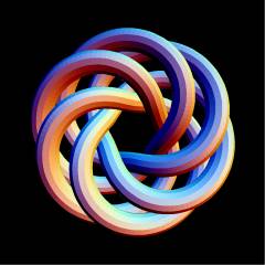
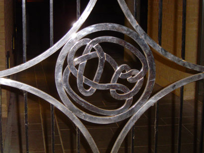
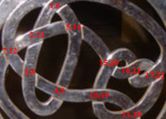
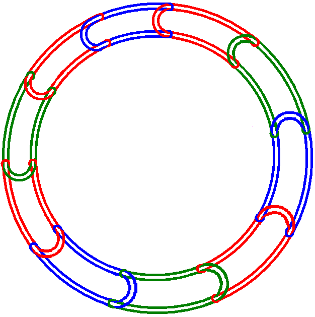
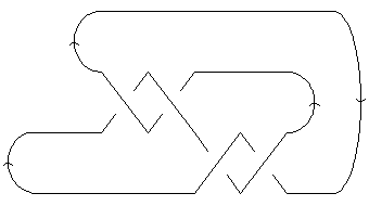
On May 1, 2007 AnonMoos asked Dror if he could identify the link in the figure on the right. So Dror typed:

In[7]:=	mva = MultivariableAlexander[L = PD[ X[1, 16, 2, 17], X[3, 15, 4, 14], X[5, 8, 6, 9], X[7, 21, 8, 20], X[9, 22, 10, 13], X[11, 2, 12, 3], X[13, 18, 14, 19], X[15, 12, 16, 1], X[17, 11, 18, 10], X[19, 4, 20, 5], X[21, 7, 22, 6] ]][t]
Out[7]=	2 -(((-1 + t[1]) (-1 + t[2]) (1 - 2 t[1] + t[1] - 2 t[2] + 2 t[1] t[2] - 2 2 2 2 2 2 t[1] t[2] + t[2] - 2 t[1] t[2] + t[1] t[2] )) / 3/2 3/2 (t[1] t[2] ))

We don't know whether our mystery link appears in the link table as is, or as a mirror, or with its two components switched. Hence we let AllPossibilities contain the multivariable Alexander polynomials of all those possibilities:

In[8]:=	AllPossibilities = Union[Flatten[ {mva, -mva} /. {{}, {t[1] -> t[2], t[2] -> t[1]}} ]]
Out[8]=	2 {-(((-1 + t[1]) (-1 + t[2]) (1 - 2 t[1] + t[1] - 2 t[2] + 2 2 2 2 2 2 t[1] t[2] - 2 t[1] t[2] + t[2] - 2 t[1] t[2] + t[1] t[2] 3/2 3/2 )) / (t[1] t[2] )), 2 ((-1 + t[1]) (-1 + t[2]) (1 - 2 t[1] + t[1] - 2 t[2] + 2 t[1] t[2] - 2 2 2 2 2 2 t[1] t[2] + t[2] - 2 t[1] t[2] + t[1] t[2] )) / 3/2 3/2 (t[1] t[2] )}

Finally, let us locate our link in the link table:

In[9]:=	Select[ AllLinks[], MemberQ[AllPossibilities, MultivariableAlexander[#][t]] & ]
Out[9]=	{Link[11, Alternating, 289]}

And just to be sure,

In[10]:=	{Jones[L][q], Jones[Link[11, Alternating, 289]][q]}
Out[10]=	-(17/2) 4 8 12 16 18 17 15 {q - ----- + ----- - ----- + ---- - ---- + ---- - ---- + 15/2 13/2 11/2 9/2 7/2 5/2 3/2 q q q q q q q 10 3/2 5/2 ------- - 7 Sqrt[q] + 3 q - q , Sqrt[q] -(5/2) 3 7 3/2 5/2 -q + ---- - ------- + 10 Sqrt[q] - 15 q + 17 q - 3/2 Sqrt[q] q 7/2 9/2 11/2 13/2 15/2 17/2 18 q + 16 q - 12 q + 8 q - 4 q + q }

Thus the mystery link is the mirror image of L11a289.

The Determinant and the Signature

(For In[1] see Setup)

In[2]:= ?KnotDet KnotDet[K] returns the determinant of a knot K.

In[3]:= ?KnotSignature KnotSignature[K] returns the signature of a knot K.

Thus, for example, the knots 5_1 and 10_132 have the same determinant (and even the same Alexander and Jones polynomials), but different signatures:

5_1

10_132

In[4]:=	KnotDet /@ {Knot[5, 1], Knot[10, 132]}
Out[4]=	{5, 5}

In[5]:=	{ Equal @@ (Jones[#][q]& /@ {Knot[5, 1], Knot[10, 132]}), Equal @@ (Alexander[#][t]& /@ {Knot[5, 1], Knot[10, 132]}) }
Out[5]=	{True, True}

In[6]:=	KnotSignature /@ {Knot[5, 1], Knot[10, 132]}
Out[6]=	{-4, 0}

In August 2005 somebody emailed Dror a question about knot colouring, which amounted to "find the first knot (other than the unknot) whose determinant is $\pm 1$". So on September 2^nd Dror typed

In[7]:=	Select[AllKnots[], Abs[KnotDet[#]] == 1 &]
Out[7]=	{Knot[0, 1], Knot[10, 124], Knot[10, 153], Knot[11, NonAlternating, 34], Knot[11, NonAlternating, 42], Knot[11, NonAlternating, 49], Knot[11, NonAlternating, 116]}

Hence the first few knots that are not $k$-colourable for any $k$ are 10_124, 10_153, K11n34, K11n42, K11n49 and K11n116.

K11n116

The Jones Polynomial

(For In[1] see Setup)

In[2]:= ?Jones Jones[L][q] computes the Jones polynomial of a knot or link L as a function of the variable q.

In Naming and Enumeration we checked that the knots 6_1 and 9_46 have the same Alexander polynomial. Their Jones polynomials are different, though:

In[3]:=	Jones[Knot[6, 1]][q]
Out[3]=	-4 -3 -2 2 2 2 + q - q + q - - - q + q q

In[4]:=	Jones[Knot[9, 46]][q]
Out[4]=	-6 -5 -4 2 -2 1 2 + q - q + q - -- + q - - 3 q q

L8a6

On links with an even number of components the Jones polynomial is a function of ${\sqrt {q}}$, and hence it is often more convenient to view it as a function of $t$, where $t^{2}=q$:

In[5]:=	Jones[Link[8, Alternating, 6]][q]
Out[5]=	-(9/2) -(7/2) 3 3 4 3/2 -q + q - ---- + ---- - ------- + 3 Sqrt[q] - 2 q + 5/2 3/2 Sqrt[q] q q 5/2 7/2 2 q - q

In[6]:=	PowerExpand[Jones[Link[8, Alternating, 6]][t^2]]
Out[6]=	-9 -7 3 3 4 3 5 7 -t + t - -- + -- - - + 3 t - 2 t + 2 t - t 5 3 t t t

The Jones polynomial attains 2110 values on the 2226 knots and links known to KnotTheory`:

In[7]:=

all = Join[AllKnots[], AllLinks[]];

In[8]:=	Length /@ {Union[Jones[#][q]& /@ all], all}
Out[8]=	{2110, 2226}

How is the Jones polynomial computed?

(See also: The Kauffman Bracket using Haskell)

The Jones polynomial is so simple to compute using Mathematica that it's worthwhile pause and see how this is done, even for readers with limited prior programming experience. First, recall (say from [Kauffman]) the definition of the Jones polynomial using the Kauffman bracket $\langle \cdot \rangle$:

[KBDef]

Failed to parse (unknown function "\slashoverback"): {\displaystyle \langle\emptyset\rangle=1; \qquad \langle\bigcirc L\rangle = (-A^2-B^2)\langle L\rangle; \qquad \langle\slashoverback\rangle = A\langle\hsmoothing\rangle + B\langle\smoothing\rangle; } $J(L)=\left.(-A^{3})^{w(L)}{\frac {\langle L\rangle }{\langle \bigcirc \rangle }}\right|_{A\to q^{1/4}},$

here $A$ is a commutative variable, $B=A^{-1}$, and $w(L)$ is the writhe of $L$, the difference $n_{+}-n_{-}$ where $n_{+}$ and $n_{-}$ count the positive Failed to parse (unknown function "\overcrossing"): {\displaystyle (\overcrossing)} and negative Failed to parse (unknown function "\undercrossing"): {\displaystyle (\undercrossing)} crossings of $L$ respectively.

PD[X[1,4,2,5], X[3,6,4,1], X[5,2,6,3]] and P[1,4] P[1,5] P[2,4] P[2,6] P[3,5] P[3,6]

Just for concreteness, let us start by fixing $L$ to be the trefoil knot shown above:

In[9]:=	L = PD[Knot[3, 1]]
Out[9]=	PD[X[1, 4, 2, 5], X[3, 6, 4, 1], X[5, 2, 6, 3]]

Our first task is to perform the replacement Failed to parse (unknown function "\slashoverback"): {\displaystyle \langle\slashoverback\rangle\to A\langle\hsmoothing\rangle + B\langle\smoothing\rangle} on all crossings of $L$. By our conventions (see Planar Diagrams) the edges around a crossing $X_{abcd}$ are labeled $a$, $b$, $c$ and $d$: Failed to parse (unknown function "\slashoverback"): {\displaystyle {}^c_d\slashoverback{}_a^b} . Labeling the smoothings Failed to parse (unknown function "\hsmoothing"): {\displaystyle (\hsmoothing, \ \smoothing)} in the same way, Failed to parse (unknown function "\hsmoothing"): {\displaystyle {}^c_d\hsmoothing{}_a^b} and Failed to parse (unknown function "\smoothing"): {\displaystyle {}^c_d\smoothing{}_a^b} , we are lead to the symbolic replacement rule $X_{abcd}\to AP_{ad}P_{bc}+BP_{ab}P_{cd}$. Let us apply this rule to $L$, switch to a multiplicative notation and expand:

In[10]:=	t1 = L /. X[a_,b_,c_,d_] :> A P[a,d] P[b,c] + B P[a,b] P[c,d]
Out[10]=	PD[A P[1, 5] P[2, 4] + B P[1, 4] P[2, 5], B P[1, 4] P[3, 6] + A P[1, 3] P[4, 6], A P[2, 6] P[3, 5] + B P[2, 5] P[3, 6]]

In[11]:=

t2 = Expand[Times @@ t1]

Out[11]=

2 A B P[1, 4] P[1, 5] P[2, 4] P[2, 6] P[3, 5] P[3, 6] + 2 2 A B P[1, 4] P[2, 5] P[2, 6] P[3, 5] P[3, 6] + 2 2 A B P[1, 4] P[1, 5] P[2, 4] P[2, 5] P[3, 6] + 3 2 2 2 B P[1, 4] P[2, 5] P[3, 6] + 3 A P[1, 3] P[1, 5] P[2, 4] P[2, 6] P[3, 5] P[4, 6] + 2 A B P[1, 3] P[1, 4] P[2, 5] P[2, 6] P[3, 5] P[4, 6] + 2 A B P[1, 3] P[1, 5] P[2, 4] P[2, 5] P[3, 6] P[4, 6] + 2 2 A B P[1, 3] P[1, 4] P[2, 5] P[3, 6] P[4, 6]

In the above expression the product P[1,4] P[1,5] P[2,4] P[2,6] P[3,5] P[3,6] represents a path in which 1 is connected to 4, 1 is connected to 5, 2 is connected to 4, etc. (see the right half of the figure above). We simplify such paths by repeatedly applying the rules $P_{ab}P_{bc}\to P_{ac}$ and $P_{ab}^{2}\to P_{aa}$:

In[12]:=	t3 = t2 //. {P[a_,b_]P[b_,c_] :> P[a,c], P[a_,b_]^2 :> P[a,a]}
Out[12]=	3 2 B P[1, 1] P[2, 2] P[3, 3] + A B P[2, 2] P[4, 4] + 3 2 2 A P[3, 3] P[4, 4] + A B P[3, 3] P[4, 4] + 3 A B P[5, 5] + 2 A B P[1, 1] P[5, 5]

To complete the computation of the Kauffman bracket, all that remains is to replace closed cycles (paths of the form $P_{aa}$ by $-A^{2}-B^{2}$, to replace $B$ by $A^{-1}$, and to simplify:

In[13]:=	t4 = Expand[t3 /. P[a_,a_] -> -A^2-B^2 /. B -> 1/A]
Out[13]=	-9 1 3 7 -A + - + A + A A

We could have, of course, combined the above four lines to a single very short program, that compues the Kauffman bracket from the beginning to the end:

In[14]:=

KB0[pd_] := Expand[ Expand[Times @@ pd /. X[a_,b_,c_,d_] :> A P[a,d] P[b,c] + 1/A P[a,b] P[c,d]] //. {P[a_,b_]P[b_,c_] :> P[a,c], P[a_,b_]^2 :> P[a,a], P[a_,a_] -> -A^2-1/A^2}]

In[15]:=	t4 = KB0[PD[Knot[3, 1]]]
Out[15]=	-9 1 3 7 -A + - + A + A A

We will skip the uninteresting code for the computation of the writhe here; it is a linear time computation, and if that's all we ever wanted to compute, we wouldn't have bothered to purchase a computer. For our $L$ the result is $-3$, and hence the Jones polynomial of $L$ is given by

In[16]:=	(-A^3)^(-3) * t4 / (-A^2-1/A^2) /. A -> q^(1/4) // Simplify // Expand
Out[16]=	-4 -3 1 -q + q + - q

L11a548

At merely 3 lines of code, our program is surely nice and elegant. But it is very slow:

In[17]:=	time0 = Timing[KB0[PD[Link[11, Alternating, 548]]]]
Out[17]=	-23 5 10 -3 5 13 17 21 25 {1., A + --- + -- + A + 6 A + 6 A + 5 A - 5 A + 4 A - A } 15 7 A A

Here's the much faster alternative employed by KnotTheory`:

In[18]:=

KB1[pd_PD] := KB1[pd, {}, 1]; KB1[pd_PD, inside_, web_] := Module[ {pos = First[Ordering[Length[Complement[List @@ #, inside]]& /@ pd]]}, pd[[pos]] /. X[a_,b_,c_,d_] :> KB1[ Delete[pd, pos], Union[inside, {a,b,c,d}], Expand[web*(A P[a,d] P[b,c]+1/A P[a,b] P[c,d])] //. { P[e_,f_]P[f_,g_] :> P[e,g], P[e_,_]^2 :> P[e,e], P[e_,e_] -> -A^2-1/A^2 } ] ]; KB1[PD[],_,web_] := Expand[web]

In[19]:=	time1 = Timing[KB1[PD[Link[11, Alternating, 548]]]]
Out[19]=	-23 5 10 -3 5 13 17 21 {0.015, A + --- + -- + A + 6 A + 6 A + 5 A - 5 A + 4 A - 15 7 A A 25 A }

(So on L11a548 KB1 is -23 5 10 -3 5 13 17 21 25 {1., A + --- + -- + A + 6 A + 6 A + 5 A - 5 A + 4 A - A }1,1

            15    7
           A     A/         -23    5    10    -3            5      13      17      21    25

{0.015, A + --- + -- + A + 6 A + 6 A + 5 A - 5 A + 4 A - A }1,1

               15    7
              A     A ~              -23    5    10    -3            5      13      17      21    25
      {1., A    + --- + -- + A   + 6 A + 6 A  + 5 A   - 5 A   + 4 A   - A  }1,1
                   15    7
                  A     A

Round[--------------------------------------------------------------------------------]

              -23    5    10    -3            5      13      17      21    25
     {0.015, A    + --- + -- + A   + 6 A + 6 A  + 5 A   - 5 A   + 4 A   - A  }1,1
                     15    7
                    A     A times faster than KB0.)

The idea here is to maintain a "computation front", a planar domain which starts empty and gradualy increases until the whole link diagram is enclosed. Within the front, the rules defining the Kauffman bracket, Equation [KBDef], are applied and the result is expanded as much as possible. Outside of the front the link diagram remains untouched. At every step we choose a crossing outside the front with the most legs inside and "conquer" it -- apply the rules of [KBDef] and expand again. As our new outpost is maximally connected to our old territory, the length of the boundary is increased in a minimal way, and hence the size of the "web" within our front remains as small as possible and thus quick to manipulate.

In further detail, the routine KB1[pd, inside, web] computes the Kauffman bracket assuming the labels of the edges inside the front are in the variable inside, the already-computed inside of the front is in the variable web and the part of the link diagram yet untouched is pd. The single argument KB1[pd] simply calls KB1[pd, inside, web] with an empty inside and with web set to 1. The three argument KB1[pd, inside, web] finds the position of the crossing maximmally connected to the front using the somewhat cryptic assignment

pos = First[Ordering[Length[Complement[List @@ #, inside]]& /@ pd]]}

KB1[pd, inside, web] then recursively calls itself with that crossing removed from pd}, with its legs added to the inside, and with web updated in accordance with [KBDef]. Finally, when pd is empty, the output is simply the value of web.

[Kauffman] ^  L. H. Kauffman, On knots, Princeton Univ. Press, Princeton, 1987.

The Coloured Jones Polynomials

KnotTheory` can compute the coloured Jones polynomial of knots and links, using the formulas in [Garoufalidis Le]:

(For In[1] see Setup)

In[2]:= ?ColouredJones ColouredJones[K, n][q] returns the coloured Jones polynomial of a knot in colour n (i.e., in the (n+1)-dimensional representation) in the indeterminate q. Some of these polynomials have been precomputed in KnotTheory`. To force computation, use ColouredJones[K,n, Program -> "prog"][q], with "prog" replaced by one of the two available programs, "REngine" or "Braid" (including the quotes). "REngine" (default) computes the invariant for closed knots (as well as links where all components are coloured by the same integer) directly from the MorseLink presentation of the knot, while "Braid" computes the invariant via a presentation of the knot as a braid closure. "REngine" will usually be faster, but it might be better to use "Braid" when (roughly): 1) a "good" braid representative is available for the knot, and 2) the length of this braid is less than the maximum width of the MorseLink presentation of the knot.

In[3]:= ColouredJones::about The "REngine" algorithm was written by Siddarth Sankaran in the summer of 2005, while the "Braid" algorithm was written jointly by Dror Bar-Natan and Stavros Garoufalidis. Both are based on formulas by Thang Le and Stavros Garoufalidis; see [Garoufalidis, S. and Le, T. "The coloured Jones function is q-holonomic." Geom. Top., v9, 2005 (1253-1293)].

Thus, for example, here's the coloured Jones polynomial of the knot 4_1 in the 4-dimensional representation of $sl(2)$:

In[4]:=	ColouredJones[Knot[4, 1], 3][q]
Out[4]=	-12 -11 -10 2 2 3 3 2 4 6 3 + q - q - q + -- - -- + -- - -- - 3 q + 3 q - 2 q + 8 6 4 2 q q q q 8 10 11 12 2 q - q - q + q

And here's the coloured Jones polynomial of the same knot in the two dimensional representation of $sl(2)$; this better be equal to the ordinary Jones polynomial of 4_1!

In[5]:=	ColouredJones[Knot[4, 1], 1][q]
Out[5]=	-2 1 2 1 + q - - - q + q q

In[6]:=	Jones[Knot[4, 1]][q]
Out[6]=	-2 1 2 1 + q - - - q + q q

4_1

3_1

In[7]:= ?CJ`Summand CJ`Summand[br, n] returned a pair {s, vars} where s is the summand in the the big sum that makes up ColouredJones[br, n][q] and where vars is the list of variables that need to be summed over (from 0 to n) to get ColouredJones[br, n][q]. CJ`Summand[K, n] is the same for knots for which a braid representative is known to this program.

The coloured Jones polynomial of 3_1 is computed via a single summation. Indeed,

In[8]:=	s = CJ`Summand[Mirror[Knot[3, 1]], n]
Out[8]=	(3 n)/2 + n CJ`k[1] + (-n + 2 CJ`k[1])/2 1 {CJ`q qBinomial[0, 0, ----] CJ`q 1 1 qBinomial[CJ`k[1], 0, ----] qBinomial[CJ`k[1], CJ`k[1], ----] CJ`q CJ`q n 1 n 1 qPochhammer[CJ`q , ----, 0] qPochhammer[CJ`q , ----, CJ`k[1]] CJ`q CJ`q n - CJ`k[1] 1 qPochhammer[CJ`q , ----, 0], {CJ`k[1]}} CJ`q

The symbols in the above formula require a definition:

In[9]:= ?qPochhammer qPochhammer[a, q, k] represents the q-shifted factorial of a in base q with index k. See Eric Weisstein's http://mathworld.wolfram.com/q-PochhammerSymbol.html and Axel Riese's www.risc.uni-linz.ac.at/research/combinat/risc/software/qMultiSum/

In[10]:= ?qBinomial qBinomial[n, k, q] represents the q-binomial coefficient of n and k in base q. For k<0 it is 0; otherwise it is qPochhammer[q^(n-k+1), q, k] / qPochhammer[q, q, k].

More precisely, qPochhammer[a, q, k] is

$(a;q)_{k}={\begin{cases}(1-a)(1-aq)\dots (1-aq^{k-1})&k>0\\1&k=0\\\left((1-aq^{-1})(1-aq^{-2})\dots (1-aq^{k})\right)^{-1}&k<0\end{cases}}$

and qBinomial[n, k, q] is

${\binom {n}{k}}_{q}={\begin{cases}{\frac {(q^{n-k+1};q)_{k}}{(q;q)_{k}}}&k\geq 0\\0&k<0.\end{cases}}$

The function qExpand replaces every occurence of a qPochhammer[a, q, k] symbol or a qBinomial[n, k, q] symbol by its definition:

In[11]:= ?qExpand qExpand[expr_] replaces all occurences of qPochhammer and qBinomial in expr by their definitions as products. See the documentation for qPochhammer and for qBinomial for details.

Hence,

In[12]:=	qPochhammer[a, q, 6] // qExpand
Out[12]=	2 3 4 5 (-1 + a) (-1 + a q) (-1 + a q ) (-1 + a q ) (-1 + a q ) (-1 + a q )

In[13]:=	First[s] /. {n -> 3, CJ`k[1] -> 2} // qExpand
Out[13]=	11 2 3 CJ`q (-1 + CJ`q ) (-1 + CJ`q )

Finally,

In[14]:= ?ColoredJones Type ColoredJones and see for yourself.

[Garoufalidis Le] ^  S. Garoufalidis and T. Q. T. Le, The Colored Jones Function is $q$-Holonomic, Georgia Institute of Technology preprint, September 2003, arXiv:math.GT/0309214.

The A2 Invariant

We compute the $A2$ (or quantum $sl(3)$) invariant using the normalization and formulas of [Khovanov], which in itself follows [Kuperberg]:

(For In[1] see Setup)

In[2]:= ?A2Invariant A2Invariant[L][q] computes the A2 (sl(3)) invariant of a knot or link L as a function of the variable q.

10_22

10_35

As an example, let us check that the knots 10_22 and 10_35 have the same Jones polynomial but different $A2$ invariants:

In[3]:=	Jones[Knot[10, 22]][q] == Jones[Knot[10, 35]][q]
Out[3]=	True

In[4]:=	A2Invariant[Knot[10, 22]][q]
Out[4]=	-12 -8 -6 -4 2 4 6 8 10 12 14 -1 + q + q + q - q + -- - q - 2 q + q - q + q + q + 2 q 18 q

In[5]:=	A2Invariant[Knot[10, 35]][q]
Out[5]=	-14 -12 -10 -8 2 2 2 6 8 10 14 16 q + q - q + q - -- + -- + q - q + q - 2 q + q - q + 4 2 q q 18 20 q + q

The $A2$ invariant attains 2163 values on the 2226 knots and links known to KnotTheory:

In[6]:=

all = Join[AllKnots[], AllLinks[]];

In[7]:=	Length /@ {Union[A2Invariant[#][q]& /@ all], all}
Out[7]=	{2163, 2226}

[Khovanov] ^  M. Khovanov, $sl(3)$ link homology I, arXiv:math.QA/0304375.

[Kuperberg] ^  G. Kuperberg, Spiders for rank 2 Lie algebras, Comm. Math. Phys. 180 (1996) 109-151, arXiv:q-alg/9712003.

Quantum knot invariants

Quantum knot invariants are calculated using Scott's QuantumGroups` Mathematica package. There is a subversion repository, and hopefully soon a documented release.

The quantum knots invariants in the Knot Atlas are normalised so the invariant of the unknot is the quantum dimension of the chosen representation.

Here we demonstrate the calculation of some quantum knot invariants. (For In[1] see Setup)

In[1]:= ?QuantumKnotInvariant QuantumKnotInvariant[Γ, V][K][q] calculates the quantum knot invariant of the knot K in the representation V of the quantum group Γ. This relies on the QuantumGroups` package, and you should look there for details of how Γ and V may be specified. Examples: QuantumKnotInvariant[Subscript[A,2], Irrep[Subscript[A,2]][{1, 0}]][Knot[5, 2]][q] QuantumKnotInvariant[Subscript[G,2], Irrep[Subscript[G,2]][{1, 0}]⊕Irrep[Subscript[G,2]][{0, 1}]][Knot[5, 2]][q]

In[2]:= QuantumKnotInvariant::about Quantum knot invariants are calculated using the mathematica package QuantumGroups`, written by Scott Morrison 2003-2006.

The Jones polynomial is a quantum knot invariant -- it corresponds to the 2-dimensional representation of the quantum group $SU(2)$, of type $A_{1}$. It's in a slightly different normalisation, however.

In[3]:=	{Jones[Knot[6,1]][q], QuantumKnotInvariant[Subscript[A,1], Irrep[Subscript[A,1]][{1}]][Knot[6,1]][q]}
Out[3]=	-4 -3 -2 2 2 -5 1 3 9 {2 + q - q + q - - - q + q , q + - - q + q } q q

In[4]:=	Simplify[(q+q^(-1))Jones[Knot[6,1]][q^(-2)] - QuantumKnotInvariant[Subscript[A,1], Irrep[Subscript[A,1]][{1}]][Knot[6,1]][q]]
Out[4]=	0

The QuantumGroups` package is capable of calculating quantum knot invariants in arbitrary representations of any quantum group. Quantum groups are specified by their Dynkin diagram. (In practice, you'll find that memory and CPU time are quite limiting.) Here are some examples.

In[5]:=	QuantumKnotInvariant[Subscript[A,2], Irrep[Subscript[A,2]][{1,1}]][Knot[7,3]][q]
Out[5]=	-76 2 2 2 2 2 6 3 2 4 -52 q + --- - --- + --- - --- + --- - --- + --- - --- + --- - q + 72 70 68 66 64 62 60 58 56 q q q q q q q q q 4 8 4 11 4 8 6 4 2 5 2 --- - --- + --- - --- + --- - --- + --- - --- + --- + --- - --- + 50 48 46 44 42 40 38 36 34 28 26 q q q q q q q q q q q 8 6 2 2 -12 --- + --- - --- + --- + q 24 20 18 16 q q q q

In[6]:=	QuantumKnotInvariant[Subscript[A,3], Irrep[Subscript[A,3]][{0,1,0}]][Knot[8,2]][q]
Out[6]=	4 6 8 10 12 18 20 22 24 1 + 2 q + 2 q + 2 q + 3 q + 2 q - 2 q - 3 q - q - q - 26 36 38 42 44 46 48 50 52 54 56 2 q + q + 2 q + q + q - q - q + q - q - q + q

In[7]:=	QuantumKnotInvariant[Subscript[G,2], Irrep[Subscript[G,2]][{1,0}]][Knot[5,2]][q]
Out[7]=	10 14 20 24 34 40 44 46 48 50 54 q + q + q + 2 q + q + q + q + 2 q - q + 2 q + q + 56 60 64 66 68 72 74 76 78 82 84 q + q + q - q - q - q - q - q - q - q - q - 88 90 92 94 96 100 q + q - q - q + q + q

In[8]:=	QuantumKnotInvariant[Subscript[D,4], Irrep[Subscript[D,4]][{0,1,0,0}]][Knot[5,1]][q]
Out[8]=	30 32 34 36 38 40 42 44 q + q + 4 q + 6 q + 10 q + 14 q + 19 q + 19 q + 46 48 50 52 56 58 60 22 q + 19 q + 14 q + 7 q - 11 q - 17 q - 24 q - 62 64 66 68 70 72 74 76 27 q - 27 q - 24 q - 18 q - 12 q - 4 q + 3 q + 9 q + 78 80 82 84 86 88 90 92 11 q + 14 q + 11 q + 9 q + 6 q + 2 q - q - q - 94 96 98 100 120 3 q - 3 q - q - q + q

In[9]:=	qDimension[Subscript[B,2]][Irrep[Subscript[B,2]][{0,1}]] /. q->1
Out[9]=	4

In[10]:=	BR[Knot[7,4]]
Out[10]=	KnotTheory`BR[4, {1, 1, 2, -1, 2, 2, 3, -2, 3}]

In[11]:=	QuantumKnotInvariant[Subscript[B,2], Irrep[Subscript[B,2]][{0,1}]][Knot[7,4]][q]
Out[11]=	-54 2 -48 -46 -44 -42 -40 -36 2 2 -q - --- + q - q + q - q + q - q + --- - --- + 50 34 32 q q q 2 2 3 2 2 -20 -18 -16 2 2 -8 --- - --- + --- - --- + --- + q + q + q + --- - --- + q - 30 28 26 24 22 12 10 q q q q q q q -6 -4 q + q

The representations in the examples above are all irreducibles, specified by their highest weight. (The QuantumGroups` package represents weights by the coordinates in the fundamental basis. Thus $Irrep[A_{3}][{0,1,0}]=\wedge ^{2}(C^{4})$, for example. We can also specify other representations, as direct sums and tensor products.

The HOMFLY-PT Polynomial

The HOMFLY-PT polynomial $H(L)(a,z)$ (see [HOMFLY] and [PT]) of a knot or link $L$ is defined by the skein relation

Failed to parse (unknown function "\overcrossing"): {\displaystyle aH\left(\overcrossing\right)-a^{-1}H\left(\undercrossing\right)=zH\left(\smoothing\right) }

and by the initial condition $H(\bigcirc )$=1.

KnotTheory` knows about the HOMFLY-PT polynomial:

(For In[1] see Setup)

In[2]:= ?HOMFLYPT HOMFLYPT[K][a, z] computes the HOMFLY-PT (Hoste, Ocneanu, Millett, Freyd, Lickorish, Yetter, Przytycki and Traczyk) polynomial of a knot/link K, in the variables a and z.

In[3]:= HOMFLYPT::about The HOMFLYPT program was written by Scott Morrison.

Thus, for example, here's the HOMFLY-PT polynomial of the knot 8_1:

In[4]:=

K = Knot[8, 1];

In[5]:=	HOMFLYPT[Knot[8, 1]][a, z]
Out[5]=	-2 4 6 2 2 2 4 2 a - a + a - z - a z - a z

It is well known that HOMFLY-PT polynomial specializes to the Jones polynomial at $a=q^{-1}$ and $z=q^{1/2}-q^{-1/2}$ and to the Conway polynomial at $a=1$. Indeed,

In[6]:=	Expand[HOMFLYPT[K][1/q, Sqrt[q]-1/Sqrt[q]]]
Out[6]=	-6 -5 -4 2 2 2 2 2 + q - q + q - -- + -- - - - q + q 3 2 q q q

In[7]:=	Jones[K][q]
Out[7]=	-6 -5 -4 2 2 2 2 2 + q - q + q - -- + -- - - - q + q 3 2 q q q

In[8]:=	{HOMFLYPT[K][1, z], Conway[K][z]}
Out[8]=	2 2 {1 - 3 z , 1 - 3 z }

8_1

L5a1

In our parametrization of the $A_{2}$ link invariant, it satisfies

$A_{2}(L)(q)=(-1)^{c}(q^{2}+1+q^{-2})H(L)(q^{-3},\,q-q^{-1})$,

where $L$ is some knot or link and where $c$ is the number of components of $L$. Let us verify this fact for the Whitehead link, L5a1:

In[9]:=

L = Link[5, Alternating, 1];

In[10]:=	Simplify[{ (-1)^(Length[Skeleton[L]]-1)(q^2+1+1/q^2)HOMFLYPT[L][1/q^3, q-1/q], A2Invariant[L][q] }]
Out[10]=	-12 -8 -6 2 -2 2 4 6 {2 - q + q + q + -- + q + q + q + q , 4 q -12 -8 -6 2 -2 2 4 6 2 - q + q + q + -- + q + q + q + q } 4 q

Other Software to Compute the HOMFLY-PT Polynomial

A C-based program running under windows by M. Ochiai can compute the HOMFLY-PT polynomial of certain knots and links with up to hundreds of crossings using "base tangle decompositions". His program, bTd, is available at [2].

References

[HOMFLY] ^  J. Hoste, A. Ocneanu, K. Millett, P. Freyd, W. B. R. Lickorish and D. Yetter, A new polynomial invariant of knots and links, Bull. Amer. Math. Soc. 12 (1985) 239-246.

[PT] ^  J. Przytycki and P. Traczyk, Conway Algebras and Skein Equivalence of Links, Proc. Amer. Math. Soc. 100 (1987) 744-748.

The Kauffman Polynomial

The Kauffman polynomial $F(K)(a,z)$ (see [Kauffman]) of a knot or link $K$ is $a^{-w(K)}L(K)$ where $w(L)$ is the writhe of $K$ (see How is the Jones Polynomial Computed?) and where $L(K)$ is the regular isotopy invariant defined by the skein relations

$L(s_{+})=aL(s),\qquad L(s_{-})=a^{-1}L(s)$

(here $s$ is a strand and $s_{\pm }$ is the same strand with a $\pm$ kink added) and

Failed to parse (unknown function "\backoverslash"): {\displaystyle L(\backoverslash)+L(\slashoverback) = z\left(L(\smoothing)+L(\hsmoothing)\right)}

and by the initial condition $L(U)=1$ where $U$ is the unknot .

KnotTheory` knows about the Kauffman polynomial:

(For In[1] see Setup)

In[2]:= ?Kauffman Kauffman[K][a, z] computes the Kauffman polynomial of a knot or link K, in the variables a and z.

In[3]:= Kauffman::about The Kauffman polynomial program was written by Scott Morrison.

Thus, for example, here's the Kauffman polynomial of the knot 5_2:

In[4]:=	Kauffman[Knot[5, 2]][a, z]
Out[4]=	2 4 6 5 7 2 2 4 2 6 2 3 3 -a + a + a - 2 a z - 2 a z + a z - a z - 2 a z + a z + 5 3 7 3 4 4 6 4 2 a z + a z + a z + a z

5_2

T(8,3)

It is well known that the Jones polynomial is related to the Kauffman polynomial via

$J(L)(q)=(-1)^{c+1}L(K)(-q^{-3/4},\,q^{1/4}+q^{-1/4})$,

where $K$ is some knot or link and where $c$ is the number of components of $K$. Let us verify this fact for the torus knot T(8,3):

In[5]:=

K = TorusKnot[8, 3];

In[6]:=	Simplify[{ (-1)^(Length[Skeleton[K]]-1)Kauffman[K][-q^(-3/4), q^(1/4)+q^(-1/4)], Jones[K][q] }]
Out[6]=	7 9 16 7 9 16 {q + q - q , q + q - q }

[Kauffman] ^  L. H. Kauffman, An invariant of regular isotopy, Trans. Amer. Math. Soc. 312 (1990) 417-471.

Finite Type (Vassiliev) Invariants

(For In[1] see Setup)

In[2]:= ?Vassiliev Vassiliev[2][K] computes the (standardly normalized) type 2 Vassiliev invariant of the knot K, i.e., the coefficient of z^2 in Conway[K][z]. Vassiliev[3][K] computes the (standardly normalized) type 3 Vassiliev invariant of the knot K, i.e., 3J''(1)-(1/36)J'''(1) where J is the Jones polynomial of K.

Thus, for example, let us reproduce Willerton's "fish" (arXiv:math.GT/0104061), the result of plotting the values of $V_{2}(K)$ against the values of $\pm V_{3}(K)$, where $V_{2}(K)$ is the (standardly normalized) type 2 invariant of $K$, $V_{3}(K)$ is the (standardly normalized) type 3 invariant of $K$, and where $K$ runs over a set of knots with equal crossing numbers (10, in the example below):

In[3]:=	ListPlot[ Join @@ Table[ K = Knot[10, k] ; v2 = Vassiliev[2][K]; v3 = Vassiliev[3][K]; {{v2, v3}, {v2, -v3}}, {k, 165} ], PlotStyle -> PointSize[0.02], PlotRange -> All, AspectRatio -> 1 ]
Out[3]=	-Graphics-

As another example, let us consider the expansion of the Jones polynomial for a knot $K$ as a power series in $x$ when we substitute the standard variable $q$ with $e^{x}$ and use the power series expansion of $e^{x}$:

$J(K)(q=e^{x})=\sum _{n=0}^{\infty }\ V_{n}(K)x^{n}$

Then, for the above coefficients we have that $V_{0}(K)=1$ and for all $n\geq 1$ $V_{n}$ is a Vassiliev invariant of type $n$ [BirmanLin]. We can see this result by using the invariant formula:

Failed to parse (unknown function "\doublepoint"): {\displaystyle V\left(\doublepoint\right)= V\left(\overcrossing\right)-V\left(\undercrossing\right)}

to check the Birman-Lin condition, which tells us that an invariant $V$ is of type $m$ if it vanishes on knots with more than $m$ double points, or self intersections (see [Bar-Natan]). Computing $V$ on knots with more than one double point by resolving one self intersection at a time, it is enough to check that $V$ vanishes on knots with $m+1$ double points:

Failed to parse (unknown function "\doublepoint"): {\displaystyle V\underbrace{ \left(\doublepoint\cdots\doublepoint\right) }_{m+1}=0}

The following two programs let us determine $V_{n}(K)$ for any integer $n$ and knot $K$:

In[4]:=

SetCrossing[K_, l_Integer, s_] := Module[ {pd, n}, pd = PD[K]; If[PositiveQ[pd[[l]]], If[s == "-", pd[[l]] = RotateRight@pd[[l]]], If[s == "+", pd[[l]] = RotateLeft@pd[[l]]]]; pd];

In[5]:=

V[K_, n_] := Series[Jones[K][Exp[x]], {x, 0, n}]; V[K_, n_, {i1_, is___}] := V[SetCrossing[K, i1, "+"], n, {is}] - V[SetCrossing[K, i1, "-"], n, {is}]; V[K_, n_, {}] := V[K, n];

The first program, SetCrossing, sets the $l^{th}$ crossing of a knot $K$ to be positive or negative depending on whether we choose $s$ to be "$+$" or "$-$". The second program uses the invariant formula to give the series expansion of the Jones polynomial of a knot $K$ discussed above, up to order $x^{n}$, where a selected list of the crossings of $K$ are taken as double points. $V_{n}(K)$ is then the coefficient of the term containing $x^{n}$.

For example, we can check that $V_{4}$ disappears on the knot 9_47 with its first five crossings taken as double points:

In[6]:=	V[Knot[9, 47], 4, {1, 2, 3, 4, 5}]
Out[6]=	V[Knot[9, 47], 4, {1, 2, 3, 4, 5}]

The knot 9_47 with its first five crossings taken as double points.

[Bar-Natan] ^ D. Bar-Natan, On the Vassiliev Knot Invariants, Topology 34 (1995) 423-472.

[BirmanLin] ^ J.S. Birman and X.-S. Lin, Knot Polynomials and Vassiliev's Invariants, Invent. Math. 111 (1993) 225-270.

Khovanov Homology

(See also: Tweaking JavaKh)

The Khovanov Homology $\operatorname {\it {KH}} (L)$ of a knot or a link $L$, also known as Khovanov's categorification of the Jones polynomial of $L$, was defined by Khovanov in [Khovanov1] (also check [Bar-Natan1]), where the notation is closer to the notation used here). It is a graded homology theory; each homology group $\operatorname {\it {KH}} ^{r}(L)$ is in itself a direct sum $\bigoplus _{j}\operatorname {\it {KH}} _{j}^{r}(L)$ of homogeneous components. Over a field one can form the two-variable "Poincaré polynomial" $\operatorname {\it {Kh}} (L)$ (which deserves the name "the Khovanov polynomial of $L$"),

$\operatorname {\it {Kh}} (L)(q,t):=\sum _{r,j}t^{r}q^{j}\dim \operatorname {\it {KH}} _{j}^{r}(L)$.

(For In[1] see Setup)

In[2]:= ?Kh Kh[L][q, t] returns the Poincare polynomial of the Khovanov Homology of a knot/link L (over a field of characteristic 0) in terms of the variables q and t. Kh[L, Program -> prog] uses the program prog to perform the computation. The currently available programs are "FastKh", written in Mathematica by Dror Bar-Natan in the winter of 2005, "JavaKh-v1", written in java (java 1.5 required!) by Jeremy Green in the summer of 2005 and "JavaKh-v2" (default), an update of "JavaKh-v1" (now requiring java 1.6) written by Scott Morrison in 2008. ("JavaKh" is also available, currently an alias for "JavaKh-v2".) The java programs are several thousand times faster than the Mathematica program, though java may not be available on some systems. "JavaKh2" also takes the option "Modulus -> p" which changes the characteristic of the ground field to p. If p==0 JavaKh works over the rational numbers; if p==Null JavaKh works over Z (see ?ZMod for the output format).

Thus for example, here's the Khovanov polynomial of the knot 5_1:

In[3]:=	kh = Kh[Knot[5, 1]][q, t]
Out[3]=	-5 -3 1 1 1 1 q + q + ------ + ------ + ------ + ----- 15 5 11 4 11 3 7 2 q t q t q t q t

The Euler characteristic of the Khovanov Homology $\operatorname {\it {KH}} (L)$ is (up to normalization) the Jones polynomial $J(L)$ of $L$. Precisely,

$\operatorname {\it {Kh}} (L)(q,-1)={\hat {J}}(L)(q):=(q+q^{-1})J(L)(q^{2})$.

Let us verify this in the case of 5_1:

In[4]:=	{kh /. t -> -1, Expand[(q+1/q)Jones[Knot[5, 1]][q^2]]}
Out[4]=	-15 -7 -5 -3 -15 -7 -5 -3 {-q + q + q + q , -q + q + q + q }

5_1

10_132

Khovanov's homology is a strictly stronger invariant than the Jones polynomial. Indeed, $J(5_{1})=J(10_{132})$ though $\operatorname {\it {Kh}} (5_{1})\neq \operatorname {\it {Kh}} (10_{132})$:

In[5]:=	{ Jones[Knot[5, 1]] === Jones[Knot[10, 132]], Kh[Knot[5, 1]] === Kh[Knot[10, 132]] }
Out[5]=	{True, False}

The algorithm presently used by KnotTheory` is an efficient algorithm modeled on the Kauffman bracket algorithm of The Jones Polynomial, as explained in [Bar-Natan3] (which follows [Bar-Natan2]). Currently, two implementations of this algorithm are available:

• FastKh: My original implementation, written in Mathematica in the winter of 2005. This implementation can be explicitly invoked using the syntax Kh[L, Program -> "FastKh"][q, t] or by changing the default behaviour of Kh by evaluating SetOptions[Kh, Program -> "FastKh"].
• JavaKh: In the summer of 2005 Jeremy Green re-implemented the algorithm in java (java 1.5 required, can be had from http://java.sun.com/) with much further care to the details, leading to an improvement factor of several thousands for large knots/links. This implementation is the default. It can also be explicitly invoked from within Mathematica using the syntax Kh[L, Program -> "JavaKh"][q, t].

In[6]:=	Options[Kh]
Out[6]=	{ExpansionOrder -> Automatic, Program -> JavaKh-v2, Modulus -> 0, KnotTheory`FastKh`Universal -> False, JavaOptions -> }

JavaKh takes an additional option, Modulus, which sets the characteristic of the ground field for the homology computations to $0$ or to a prime $p$. Thus for example, the following four In lines imply that the Khovanov homology of the torus knot T(6,5) has both 3 torsion and 5 torsion, but no 7 torsion:

In[7]:=

T65 = TorusKnot[6, 5]; kh = Kh[T65][q, t];

In[8]:=	Kh[T65, Modulus -> 3][q, t] - kh
Out[8]=	43 13 43 14 q t + q t

In[9]:=	Kh[T65, Modulus -> 5][q, t] - kh
Out[9]=	35 10 35 11 39 11 39 12 q t + q t + q t + q t

In[10]:=	Kh[T65, Modulus -> 7][q, t] - kh
Out[10]=	0

T(6,5)

The following further example is a bit tougher. It takes my computer nearly an hour and some 256Mb of memory to find that the Khovanov homology of the 48-crossing torus knot T(8,7) has 3, 5 and 7 torsion but no 11 torsion:

In[11]:= ?JavaOptions JavaOptions is an option to Kh. Kh[L, Program -> "JavaKh2", JavaOptions -> jopts] calls java with options jopts. Thus for example, JavaOptions -> "-Xmx256m" sets the maximum java heap size to 256MB - useful for large computations.

In[12]:=

SetOptions[Kh, JavaOptions -> "-Xmx256m"];

In[13]:=

T87 = TorusKnot[8, 7]; kh = Kh[T87][q, t];

In[14]:=	Factor[Kh[T87, Modulus -> 3][q, t] - kh]
Out[14]=	79 25 q t (1 + t)

In[15]:=	Factor[Kh[T87, Modulus -> 5][q, t] - kh]
Out[15]=	61 11 12 10 14 12 18 13 q t (1 + t) (1 + q t + q t + q t )

In[16]:=	Factor[Kh[T87, Modulus -> 7][q, t] - kh]
Out[16]=	61 14 8 6 12 7 10 8 14 9 q t (1 + t) (1 + q t + q t + q t + q t )

In[17]:=	Factor[Kh[T87, Modulus -> 11][q, t] - kh]
Out[17]=	0

JavaKh also works over the integers:

In[18]:= ?ZMod ZMod[m] denotes the cyclic group Z/mZ. Thus if m=0 it is the infinite cyclic group Z and if m>0 it is the finite cyclic group with m elements. ZMod[m1, m2, ...] denotes the direct sum of ZMod[m1], ZMod[m2], ... .

For example, the 22nd homology group over ${\mathbb {Z} }$ of the torus knot T(8,7) at degree 73 is the 280 element torsion group ${\mathbb {Z} }_{2}\oplus {\mathbb {Z} }_{4}\oplus {\mathbb {Z} }_{5}\oplus {\mathbb {Z} }_{7}$:

In[19]:=	Coefficient[Kh[T87, Modulus -> Null][q, t], t^22 * q^73]
Out[19]=	ZMod[2, 4, 5, 7]

T(8,7) is currently not on the Knot Atlas. Let us see what it looks like:

In[20]:=	Show[TubePlot[TorusKnot[8, 7]]]
Out[20]=	-Graphics3D-

Finally, JavaKh may also be run outside of Mathematica, as the following example demonstrates:

drorbn@coxeter:.../KnotTheory: cd JavaKh
drorbn@coxeter:.../KnotTheory/JavaKh: java JavaKh
PD[X[3, 1, 4, 6], X[1, 5, 2, 4], X[5, 3, 6, 2]]
"+ q^1t^0 + q^3t^0 + q^5t^2 + q^9t^3 "

(Type java JavaKh -help for some further help).

(Warning, as of August 2008, you need to include the .jar files in JavaKh/jars on the classpath. If this causes confusion, ask Scott for a script that manages this automatically, or look at p. 29 of [3] for an example.)

Universal Khovanov homology, and reduced homology

The KnotTheory` package can now compute the universal homology over $\mathbb {Q}$, the reduced homology over $\mathbb {Q}$ as well as directly computing the s-invariant. Type ?UniversalKh, ?KhReduced or ?sInvariant for more information.

The output of UniversalKh is a $\mathbb {N} [q,t]$-linear combination of symbols KhE and KhC[n] for some positive integer $n$. The coefficients of these symbols are individually knot invariants, capturing all of the information in the spectral sequences (over $\mathbb {Q}$) for both unreduced and reduced homology.

The s-invariant can be extracted from the output of UniversalKh: the coefficient of KhE is exactly $q^{s}$.

The usual 2-variable Khovanov polynomial Kh[K][q,t] can be recovered from UniversalKh[K][q,t] by using the substitution rules

   {KhE->q+q^-1,KhC[1]->t^-1 q^-3+ q^1,KhC[n_]/;n>=2:>(q+q^-1)(t^-1 q^(-2n)+1)};

and similarly the reduced Khovanov polynomial KhReduced[K][q,t] is actually produced by substituting UniversalKh[K][q,t] using the rules

   {KhE->q^-1,KhC[n_]:>t^-1 q^(-2n-1)+q^-1};

Unfortunately, much of the mathematics behind UniversalKh is not in print. There's some explanation in Scott's slides from Kyoto.

UniversalKh also takes the same JavaOptions option described above for Kh, which may be necessary to allow enough memory for large computations.

References

August 2002, Toronto: Mikhail Khovanov explaining his paper [Khovanov2].

[Bar-Natan1] ^  D. Bar-Natan, On Khovanov's categorification of the Jones polynomial, Algebraic and Geometric Topology 2-16 (2002) 337-370, arXiv:math.GT/0201043.

[Bar-Natan2] ^  D. Bar-Natan, Khovanov's Homology for Tangles and Cobordisms, Geometry and Topology 9-33 (2005) 1443-1499, arXiv:math.GT/0410495.

[Bar-Natan3] ^  D. Bar-Natan, I've Computed Kh(T(9,5)) and I'm Happy, talk given at Knots in Washington XX, George Washington University, February 2005.

[Khovanov1] ^  M. Khovanov, A categorification of the Jones polynomial, arXiv:math.QA/9908171.

[Khovanov2] ^  M. Khovanov, An invariant of tangle cobordisms, arXiv:math.QA/0207264.

See also A Khovanov homology bibliography.

Heegaard Floer Knot Homology

In 2007, Jean-Marie Droz of the University of Zurich (working along with Anna Beliakova) wrote a Python program to compute the (hat-version) Heegaard-Floer Knot Homology ${\widehat {\operatorname {HFK} }}(K)$ of a knot $K$ (see arXiv:0803.2379). His program is integrated into KnotTheory`, though to run it, you must have Python as well as the Python library Psyco installed on your system.

(For In[1] see Setup)

In[1]:= ?HFKHat HFKHat[K][t,m] returns the Poincare polynomial of the Heegaard-Floer Knot Homology (hat version) of the knot K, in the Alexander variable t and the Maslov variable m.

In[2]:= HFKHat::about The Heegaard-Floer Knot Homology program was written by Jean-Marie Droz in 2007 at the University of Zurich, based on methods of Anna Beliakova's arXiv:07050669.

8_19	in Arc Presentation

The Heegaard-Floer Knot Homology is a categorification of the Alexander polynomial. Let us test that for the knot 8_19:

In[3]:=	hfk = HFKHat[K = Knot[8, 19]][t, m]
Out[3]=	2 -3 m 5 2 6 3 m + t + -- + m t + m t 2 t

In[4]:=	{hfk /. m -> -1, Alexander[K][t]}
Out[4]=	-3 -2 2 3 -3 -2 2 3 {1 + t - t - t + t , 1 + t - t - t + t }

The knot 8_19 is the first knot in the Rolfsen Knot Table whose Heegaard-Floer Knot Homology is not "diagonal". Let us test that. The homology ${\widehat {\operatorname {HFK} }}(K)$ is "on diagonal", iff its Poincare polynomial, evaluated at $m=1/t$, is a monomial:

In[5]:=	Select[AllKnots[{3, 8}], (Head[HFKHat[#][t, 1/t]] == Plus) &]
Out[5]=	{Knot[8, 19]}

In[6]:=	hfk /. m -> 1/t
Out[6]=	4 -2 -- + t 3 t

K11n34

K11n42

The (mirrored) Conway knot K11n34 and the (mirrored) Kinoshita-Terasaka knot K11n42 are a mutant pair, and are notoriously difficult to tell apart. Let us check that an array of standard knot polynomials fails to separate them, yet ${\widehat {\operatorname {HFK} }}$ succeeds:

In[7]:=	K1 = Knot["K11n34"]; K2 = Knot["K11n42"]; test[invt_] := (invt[K1] =!= invt[K2]); test /@ { Alexander, MultivariableAlexander, Jones, HOMFLYPT, Kauffman, Kh, HFKHat }
Out[7]=	{False, False, False, False, False, False, True}

Indeed,

In[8]:=	{HFKHat[K1][t, m], HFKHat[K2][t, m]}
Out[8]=	2 1 1 3 3 3 3 {3 + - + ----- + ----- + ----- + ----- + ---- + --- + 3 t + 3 m t + m 4 3 3 3 3 2 2 2 2 m t m t m t m t m t m t 2 2 2 2 3 3 3 3 m t + 3 m t + m t + m t , 6 1 1 4 4 2 2 2 7 + - + ----- + ----- + ---- + --- + 4 t + 4 m t + m t + m t } m 3 2 2 2 2 m t m t m t m t

On July 6, 2006, User:AnonMoos asked User:Drorbn if he could identify the knot in the left hand side picture below. At the time it was impossible using the tools available with KnotTheory` - using any of many invariants, the answer can be found to be either the mirror of K11n34 or the mirror of K11n42, but KnotTheory` couldn't tell which one it is (though of course, it is possible to do it "by hand"). The 2007 addition ${\widehat {\operatorname {HFK} }}$ does the job, though. Indeed, we first extract the mystery knot's DT (Dowker-Thistlethwaite) Code using the picture on the right hand side below, then compute ${\widehat {\operatorname {HFK} }}$, and then search for it within the ${\widehat {\operatorname {HFK} }}$'s of all knots with up to 11 crossings:

In[9]:=

K3 = DTCode[6, 8, 14, 12, 4, -18, 2, -20, -22, -10, -16];

In[10]:=	H = HFKHat[Mirror[K3]][t, m]
Out[10]=	2 1 1 3 3 3 3 3 + - + ----- + ----- + ----- + ----- + ---- + --- + 3 t + 3 m t + m 4 3 3 3 3 2 2 2 2 m t m t m t m t m t m t 2 2 2 2 3 3 3 3 m t + 3 m t + m t + m t

In[11]:=	Select[AllKnots[], HFKHat[#][t, m] == H &]
Out[11]=	{Knot[11, NonAlternating, 34]}

And so the mystery knot is the Conway knot, the mirror of K11n34.

R-Matrix Invariants

KnotTheory` can compute knot and link invariants associated with matrix solutions of the Yang-Baxter equation, using the program REngine:

(For In[1] see Setup)

In[1]:= ?REngine REngine[K, Rp, Rn, Mcupl, Mcupr, Mcapl Mcapr] returns the invariant associated with the given R-matrices (Rp for positive crossings, Rn for negative crossings) and oriented creation and annihilation M matrices, of the oriented knot or link K. See the Manual for details of convention. Note that REngine does not verify that the given matrices actually define an invariant, use TestRMatrix[..] for this purpose.

In[2]:= REngine::about REngine was written by Siddarth Sankaran at the University of Toronto, in the summer of 2005

In more detail, let $V$ be a free module of finite rank over a commutative ring, and let $R,{\bar {R}}\in End(V\otimes V)$ be invertible. Further, let there be invertible endomorphisms $M_{\leftarrow },M_{\rightarrow },M^{\leftarrow },M^{\rightarrow }\in End(V)$; these correspond to McupL, McupR, McapL, and McapR respectively. Fixing a basis of V, we can regard all of these endomorphisms as matrices.

The following notation is useful: for $n=dim(V)$, $R_{ab}^{cd}$ refers to the element of R in row $n(c-1)+d$ and column $n(a-1)+b$.

For an oriented knot or link $K$, REngine returns the product $\tau (K)$, which is computed as follows:

1. Find a Morse link presentation of $K$ such that it is composed only of crossings of the X[k, Over/Under, Down, Down] variety; this is accomplished by adding caps and cups where necessary.
2. Label the edges in between events in the Morse link presentation of $K$.
3. Associate each event with one of the matrices as shown, with the indices given by the labelling:
   • X[k, Over, Down, Down]:$\Rightarrow R_{ab}^{cd}$ (positive crossing)
   • X[k, Under,Down, Down]: $\Rightarrow {\bar {R}}_{ab}^{cd}$ (negative crossing)
   • Cup[k, k+1]: $\Rightarrow {M_{\rightarrow }}_{ab}$
   • Cup[k, k-1]: $\Rightarrow {M_{\leftarrow }}_{ab}$
   • Cap[k, k+1]: $\Rightarrow {M^{\rightarrow }}_{ab}$
   • Cap[k, k-1]: $\Rightarrow {M^{\leftarrow }}_{ab}$
4. Define $\tau (K)$ as the result of taking the product of the matrices associated with the elements of K, and summing over repeated indices; each sum runs from 1 to $n=dim(V)$.

A trefoil knot

As an example, let K be the trefoil as shown, with the chosen axis upwards, and the strands going down through all the crossings. Then $\tau (K)=\sum {M_{\leftarrow }}_{ab}{M_{\rightarrow }}_{cd}R_{bc}^{ef}R_{ef}^{gh}R_{gh}^{ij}{M^{\rightarrow }}_{ai}{M^{\leftarrow }}_{jd}$

where the summation is carried out on all the indices a through i, each ranging from 1 to n.

Determining that $\tau (K)$ is actually an invariant is simply a matter of checking the equality of the outcomes of Reidemeister moves in various configurations and orientations, as well as a few 'topological' moves. Note that REngine does not perform any checks, while the utility TestRMatrix performs the tests required to determine regular isotopy.

Let's use the REngine to find the Jones polynomial of the trefoil. The R and M matrices for the Jones polynomial, in the indeterminate t, are as follows:

$R={\begin{pmatrix}t^{1/2}&0&0&0\\0&0&t&0\\0&t&t^{1/2}-t^{3/2}&0\\0&0&0&t^{1/2}\end{pmatrix}},{\bar {R}}=R^{-1}$

$M^{\leftarrow }=M^{\rightarrow }=M_{\leftarrow }=M_{\rightarrow }={\begin{pmatrix}0&t^{-1/4}\\t^{1/4}&0\end{pmatrix}}$

Putting these definitions into Mathematica, we run the REngine on the trefoil. Note that the Jones polynomial is usually normalized so that the polynomial of the unknot 0_1 is 1, hence the term on the denominator.

In[3]:=

r={{Sqrt[t], 0, 0, 0},{0, 0, t, 0},{0,t, Sqrt[t] - t^(3/2), 0}, {0,0,0,Sqrt[t]}}; rb = Inverse[r]; mcupl=mcapl=mcupr=mcapr={{0, t^(-1/4)},{t^(1/4), 0}};

In[4]:=	jones = REngine[Knot[3,1], r, rb, mcupl, mcapl, mcupr, mcapr] / REngine[Knot[0,1], r, rb, mcupl, mcapr, mcupr, mcapr] //Apart
Out[4]=	-4 -3 1 -t + t + - t

See also

See also QuantumGroups`, a Mathematica package by Scott Morrison, now included in KnotTheory`, which computes arbitrary quantum knot invariants. (For now, it only uses braid representations, not morse link representations.)

Extras Included with KnotTheory`

The package KnotTheory` contains a few extras that are not directly related to knot theory.

• Drawing with TubePlot
  • Standalone_TubePlot
• Using the LinKnot package
• WikiLink
• QuantumGroups`

Drawing with TubePlot

(For In[1] see Setup)

In[2]:= ?TubePlot TubePlot[gamma, {t, t0, t1}, r, opts] plots the space curve gamma with the variable t running from t0 to t1, as a tube of radius r. The available options are TubeSubdivision, TubeFraming and TubePlotPrelude. All other options are passed on to Graphics3D. TubePlot[TorusKnot[m, n], opts] produces a tube plot of the (m,n) torus knot.

Thus here's a thin unknot:

In[3]:=	Show[TubePlot[{Cos[t], Sin[t], 0}, {t, 0, 2Pi}, 0.1]]
Out[3]=	-Graphics3D-

In[4]:= ?TubeSubdivision TubeSubdivision is an option for TubePlot. TubePlot[__, TubeSubdivision -> {l, m} draws the tube subdivided to l pieces lengthwise and m pieces around. The default is TubeSubdivision -> {50, 12}.

In[5]:= ?TubeFraming TubeFraming is an option for TubePlot. TubePlot[gamma, {t, __}, _, TubeFraming -> n] sets the framing of the tube (visible when TubeSubdivision -> {l, m} with small m) to be the vector n, which in itself may be a function of t. Thus TubeFraming -> {0,0,1} is "blackboard framing". TubeFraming -> Normal (default) uses the normal vector of the curve gamma.

In[6]:= ?TubePlotPrelude TubePlotPrelude is an option for TubePlot. Its value is passed to Graphics3D before the main part of the plot, allowing to set various graphics options. For example, TubePlotPrelude -> EdgeForm[{}] will suppress the drawing of edges between the polygons making up the tube. The default is TubePlotPrelude -> {}.

Here's the same unknot, made thicker and not as smooth:

In[7]:=	Show[TubePlot[ {Cos[t], Sin[t], 0}, {t, 0, 2Pi}, 0.3, TubeSubdivision -> {6, 3} ]]
Out[7]=	-Graphics3D-

Let's play with the framing now:

In[8]:=	Show[TubePlot[ {Cos[t], Sin[t], 0}, {t, 0, 2Pi}, 0.2, TubeSubdivision -> {50, 2}, TubeFraming -> {Cos[2t]Cos[t], Cos[2t]Sin[t], Sin[3t]} ]]
Out[8]=	-Graphics3D-

Here's an example that uses a prelude and passes options on to Graphics3D:

In[9]:=	Show[TubePlot[ {Cos[2t], Sin[2t], 0} + 0.5{Cos[3t]Cos[2t], Cos[3t]Sin[2t], -Sin[3t]}, {t, 0, 2Pi}, 1/3, TubeSubdivision -> {280, 12}, TubeFraming -> {0,0,1}, TubePlotPrelude -> EdgeForm[{}], Boxed -> False, ViewPoint -> {0,0,1} ]]
Out[9]=	-Graphics3D-

The last example serves as the basis for the definition of TubePlot[TorusKnot[m, n]]. Here's a final example:

In[10]:=	Show[TubePlot[TorusKnot[3, 5]]]
Out[10]=	-Graphics3D-

Standalone TubePlot

There may be some independent interest in the routine TubePlot, and hence it is available also as an independent package. Here it is: TubePlot.m (File:TubePlot.m).

Using the LinKnot package

The Mathematica package LinKnot is a combination of two packages. The first, "Knot2000" was written by M. Ochiai and N. Imafuji. This was extended to the package LinKnot by S. Jablan and R. Sazdanovic. This package provides many useful things KnotTheory can't do natively; for example, it can interpret Conway notation, and, at least on Windows machines, provides nice graphics for knots, and a graphical interface for drawing knots by hand.

(LinKnot also has a webMathematica interface!)

There are two ways LinKnot can be used along with KnotTheory`:

• As a "subcontractor": LinKnot is mostly hidden and wrapper functions are provided to access some of its functionality from within KnotTheory`.
• In parallel: everything from both packages is visible.

The advantage for the first approach is that the interface to LinKnot is then consistent with the conventions used by KnotTheory` and the Mathematica name space remains less cluttered. The advantage of the second approach is obvious - with it, all the functionality of LinKnot is available, and not just the parts for which wrapper functions are provided within KnotTheory`.

Using LinKnot as a "subcontractor"

To use LinKnot from within KnotTheory, download the file LinKnot.zip from the LinKnot site or from our mirror. Unzip and install the content of LinKnot.zip wherever you like, and within Mathematica issue a command like

(For In[1] see Setup)

In[2]:=

AppendTo[$Path, "/path/to/LinKnots.m"];

After you've done this, everything should just work. (LinKnot will only be loaded when necessary, and there might be a short delay when this happens.) If everything doesn't just work, please complain to Scott.

In case of problems, you may find it helpful to explicitly set the path in which you've installed LinKnot (although KnotTheory tries to do this itself). Simply set LinKnotDirectory[].

In[3]:= ?LinKnotDirectory LinKnotDirectory[] contains the path to the ''LinKnot'' package. It must be set correctly in order for all the (Windows only) MathLink components of ''LinKnot'' to be usable. It can be overriden by the user.

Using LinKnot in parallel with KnotTheory`

To use LinKnot in parallel with KnotTheory`, you should download LinKnot.zip from the LinKnot site (a full LinKnot manual page ManualK2KC.nb is in the zip file, and the main file is the mathematica notebook K2KL.nb). After downloading the file LinKnot.zip:

1. Extract LinKnot.zip anywhere (e.g., to the local disc "C:\"). It will automatically create a new folder LinKnot.
2. Set the directory to LinKnot, add the path to KnotTheory` to the Mathematica $Path, and run:

SetDirectory["/path/to/LinKnot/"];
<< LinKnots`
AppendTo[$Path, "Path to KnotTheory"];
<< KnotTheory`

For example, if LinKnot is installed in "C:\LinKnot" and KnotTheory` is installed at "C:\KnotTheory", run:

SetDirectory["C:\\LinKnot"];
<< LinKnots`
AppendTo[$Path, "C:\\"];
<< KnotTheory`

Then you can work with the both programs KnotTheory` and LinKnot.

If you need to have the complete program LinKnot visible (with the usage, description of all LinKnot functions, etc.) and run together KnotTheory` and LinKnot, you can open the file K2KL.nb from the directory LinKnot and run the same command as before.

After you've done this, everything should just work. If everything doesn't just work, please complain to S. Jablan (jablans@yahoo.com).

Further usage notes by Jablans

If you have any problem with running LinKnot (as a separate program) please do the following:

1. in your Mathematica directory (e.g., C:\Program Files\Wolfram Research\Mathematica\5.0) make a new folder named LinKnot;
2. extract the contents of the file LinKnot.zip into the directory LinKnot;
3. open the "Mathematica" notebook K2KL.nb that you will find in the directory LinKnot;
4. run the first line:

SetDirectory["LinKnot"]
<< LinKnots.m

Then you can fix the appropriate path and work with KnotTheory and LinKnot as well.

See also

See also Extending/Modifying KnotTheory`#Lessons learnt from integrating LinKnot` for technical details on how LinKnot` and KnotTheory` were integrated.

WikiLink

WikiLink is actually two separate things; firstly, a java class for interfacing with a mediawiki server, and secondly, a Mathematica package providing a wrapper around this. This page documents the Mathematica package, while the java class, and its addition functionality, will be documented elsewhere.

WikiLink is available as a standalone package, suitable for use with any Mediawiki installation, and is included in the KnotTheory` package.

License

WikiLink.nb, WikiLink.m and wikilink.jar are copyright Scott Morrison, available under your choice of the MIT, Apache or GPL licenses. The other components are copyright by other parties, all available under the Apache license.

Download

If you already have KnotTheory` installed, there's no need to install anything. The functionality of WikiLink is available as soon as you open KnotTheory`.

Otherwise, download WikiLink.zip. Unzip this anywhere you like. This will create a subdirectory called WikiLink, containing (at least) these files:

Filename	Description
mathematica/WikiLink.nb	The Mathematica notebook containing wrapper function definitions.
mathematica/WikiLink.m	The Mathematica package automatically generated from WikiLink.nb.
wikilink.jar	The WikiLink java classes and source code.
jars/jdom.jar jars/commons-httpclient-3.0-rc2.jar jars/commons-codec-1.3.jar jars/commons-lang-2.1.jar jars/commons-logging.jar	Libraries (all available under either GPL or the Apache license) required by wikilink.jar

Importing the package in Mathematica

If you're not using KnotTheory`, first, you'll need to set some paths, so WikiLink` can find the java files it needs. You need to add the "mathematica/" subdirectory of the WikiLink distribution to the Mathematica $Path.

In[1]:=

WikiLinkPath = "/path/to/WikiLink/mathematica/";

In[2]:=

AppendTo[$Path, WikiLinkPath];

In[3]:=

<<WikiLink`

If you've already loaded KnotTheory` (e.g., with the statement <<KnotTheory`), you can simply begin at this point.

We then try to connect to the wiki. Executing this line will prompt you for a username and password.

In[6]:=

CreateWikiConnection[ "http://katlas.math.toronto.edu/w/index.php", InputString["Enter Your Username:"], InputString["Enter Your Password:"] ]

The function WikiUserName[] checks that we're logged in

In[4]:= ?WikiUserName WikiUserName[] returns either the name of the user you are logged in as, your IP address if you're not logged in, or $Failed if something more complicated has happened!

In[5]:=	WikiUserName[]
Out[5]=	ScottManualRobot

Usage

WikiLink` provides functions for checking your login status, getting and setting pages, as well as transparently extending some of Mathematica's string manipulation functions to wiki pages.

In[6]:= ?WikiUserName WikiUserName[] returns either the name of the user you are logged in as, your IP address if you're not logged in, or $Failed if something more complicated has happened!

In[7]:= ?WikiGetPageText WikiGetPageText[pagename] returns the raw text of the specified page.

In[8]:= ?WikiSetPageText WikiSetPageText[pagename, text] overwrites the contents of the specificied page with the given text. WikiSetPageText[pagename, text, summary] overwrites the contents of the specificied page with the given text and notes summary in the change log.

In[9]:= ?WikiSetPageTexts WikiSetPageText[{{pagename1, text1},{pagename2,text2},...}] efficiently sets multiple pages, by first checking which texts are already up to date.

In[10]:= ?WikiUploadFile WikiUploadFile[name, description] uploads the specified file to the wiki.

Thus for example after

In[11]:=	WikiSetPageText["Sandbox", "A robotic edit, at 19:39, 31-August-2005."]
Out[11]=	True

we get

In[12]:=	WikiGetPageText["Sandbox"]
Out[12]=	A robotic edit, at 19:39, 31-August-2005.

The function WikiSetPageTexts is most useful for batch uploads, as it does considerably more error checking, and filters out edits which won't change the page text. It takes as argument a list of {"title", "text"} pairs, and returns a list of those pairs which failed.

In[13]:=	WikiSetPageTexts[{{"Sandbox", "A robotic edit, by --~~"<>"~~"}, {"Sandbox2", "The determinant of the knot [[3_1]] is 3."}}]
Out[13]=	{}

In[14]:=	WikiGetPageText["Sandbox2"]
Out[14]=	The determinant of the knot [[3_1]] is 3.

String manipulation functions

WikiLink` provides functions WikiPageMatchQ, WikiPageFreeQ, WikiStringReplace and WikiStringCases. Each function works likes its usual Mathematica partner, StringMatchQ, StringFreeQ, StringReplace or StringCases. Instead of providing a string, or list of strings, as the first argument, you should give the name of a page, or a list of names.

You can use these to perform all sorts of editing tricks.

In[15]:=	WikiPageMatchQ[{"Sandbox", "Sandbox2"}, "determinant"]
Out[15]=	{False, False}

In[16]:=	WikiPageFreeQ[{"Sandbox", "Sandbox2"}, "[["~~(DigitCharacter..)~~"_"~~(DigitCharacter..)~~"]]"]
Out[16]=	{True, False}

In[17]:=	WikiStringCases[{"Sandbox", "Sandbox2"}, "[["~~ShortestMatch[__]~~"]]"]
Out[17]=	{{Sandbox, {[[User:ScottManualRobot|ScottManualRobot]]}}, {Sandbox2, {[[3_1]]}}}

In[18]:=	WikiStringReplace[{"Sandbox", "Sandbox2"}, "robotic edit"->"robotic edit (using WikiLink`)]
Out[18]=	$Failed

In[19]:=	WikiGetPageTexts[{"Sandbox", "Sandbox2"}]
Out[19]=	{{Sandbox, A robotic edit, by\ --[[User:ScottManualRobot|ScottManualRobot]] 14:54, 18 Feb 2006\ (EST)}, {Sandbox2, The determinant of the knot [[3_1]] is 3.}}

Troubleshooting

The instruction ShowJavaConsole[] will bring up a window in which some debugging information is displayed.

Compatibility

WikiLink (with some modifications made in July 2007) appears to work with mediawiki 1.10.1. Bug reports appreciated!

WikiLink has been tested against mediawiki 1.4.5beta3 and 1.4.7.

WikiLink has known issues on mediawiki 1.5.0. Retrieving multiple pages at once is broken. This appears to be a mediawiki bug, and will not be fixed. The same problem does not occur on mediawiki 1.5.8. --Scott 10:56, 27 Mar 2006 (EST)

I expect WikiGetPage text to continue working in mediawiki 1.5 and beyond, because it uses the stable interface Special:Export. Logging in and setting pages will quite likely break in the next version. If you've tried this, please let me know about your experiences. I'm hoping that soon (1.5?) Special:Import will become available, and I can switch to using this. --Scott 15:57, 31 Aug 2005 (EDT)

Todo

I'd love to create an Ant task which allows uploading a file to a wiki. We could then use this in build scripts for KnotTheory, etc. --Scott 04:07, 17 Sep 2005 (EDT)

See Also

All of the Mathematica notebooks in Category:Knot Atlas Maintenance Software rely on WikiLink, and so are good examples of how to use it.

You may also be interested in the Wikipedia page on mediawiki bots, and in particular the Python Wikipedia Robot Framework.

QuantumGroups`

Download

For now, QuantumGroups` is only available from its SVN repository (about SVN), or as a subpackage of KnotTheory`.

Installation

If you're planning on using QuantumGroup` from inside KnotTheory`, you just have to execute <<QuantumGroups` after loading the KnotTheory` package. Otherwise, you'll first need to add it to the path (that is, add the directory containing QuantumGroups.m to $Path), and then execute <<QuantumGroups`.

Examples of use

Root systems

Weyl groups

Weight multiplicities and tensor product decomposition

Explicit bases, and matrix presentations

Generators and relations of quantum groups

Action of the braided coxeter group on the quantum group

Quantum root operators

R-matrices

Quantum knot invariants

If you've installed the KnotTheory` package, there's a very simple interface for computing quantum knot invariants. (Be warned however, that without precomputed data files installed, this will recompute everything from scratch, for each knot, and thus be extremely slow.)

In[]:=	QuantumKnotInvariant[A2, Irrep[A2][{1,1}]][Knot[8,19]][q]
Out[]=	2 -68 2 2 -60 4 4 4 2 4 6 7 8 6 4 -36 2 4 6 7 --- - q - --- - --- + q + --- + --- + --- + --- - --- - --- - --- - --- - --- - --- - q + --- + --- + --- + --- + 72 66 64 58 56 54 52 48 46 44 42 40 38 34 32 30 28 q q q q q q q q q q q q q q q q q 6 4 2 -20 --- + --- + --- + q 26 24 22 q q q

Things to do

• PBW basis for the quantum group
• Special bases for representations
  • Gelfand-Tsetlin basis for type A
  • Canonical bases
  • Web bases for $A_{1}$, $A_{2}$, $B_{2}$, $G_{2}$

Lightly Documented Features

(For In[1] see Setup)

In[2]:= ?NumberOfKnots NumberOfKnots[n] returns the number of knots with n crossings. NumberOfKnots[n, Alternating|NonAlternating] returns the number of knots of the specified type.

In[3]:=	NumberOfKnots[16, NonAlternating]
Out[3]=	1008906

In[4]:= ?AlternatingQ AlternatingQ[D] returns True iff the knot/link diagram D is alternating.

Among the knots with up to 11 crossings, 564 are alternating and 238 are not:

In[5]:=	Total[AlternatingQ /@ AllKnots[{0,11}]]
Out[5]=	238 False + 564 True

A Sample KnotTheory` Session

Setup

The first step is to load KnotTheory` as in the Setup section:

In[1]:= << KnotTheory`

Loading KnotTheory` (version of September 14, 2005, 13:37:36)...

8_17

K11a231

L8n6

T(7,5)

Let us now introduce the four star knots that will accompany us throughout this session:

In[2]:=

K = Knot[8, 17]; K11 = Knot[11, Alternating, 231]; L = Link[8, NonAlternating, 6]; TK = TorusKnot[7,5];

Presentations, Graphical Output and Tube Plots

Planar Diagrams

In[3]:=	PD[K]
Out[3]=	PD[X[6, 2, 7, 1], X[14, 8, 15, 7], X[8, 3, 9, 4], X[2, 13, 3, 14], X[12, 5, 13, 6], X[4, 9, 5, 10], X[16, 12, 1, 11], X[10, 16, 11, 15]]

Gauss Codes

In[4]:=	{GaussCode[K], GaussCode[L]}
Out[4]=	{GaussCode[1, -4, 3, -6, 5, -1, 2, -3, 6, -8, 7, -5, 4, -2, 8, -7], GaussCode[{1, -7, 2, -8}, {-5, 4, -6, 3}, {7, -1, -4, 5, 8, -2, -3, 6}]}

DT (Dowker-Thistlethwaite) Codes

In[5]:=	DTCode[K]
Out[5]=	DTCode[6, 8, 12, 14, 4, 16, 2, 10]

Braid Representatives

In[6]:=	br = BR[K]
Out[6]=	BR[3, {-1, -1, 2, -1, 2, -1, 2, 2}]

In[7]:=	{First[br], Crossings[br], BraidIndex[K]}
Out[7]=	{3, 8, 3}

Drawing Braids

In[8]:=	Show[BraidPlot[br]]
Out[8]=	-Graphics-

Drawing MorseLink Presentations

In[9]:=	Show[DrawMorseLink[K]]
Out[9]=	-Graphics-

In[10]:=	Show[DrawMorseLink[L]]
Out[10]=	-Graphics-

Drawing with TubePlot

In[11]:=	Show[TubePlot[TK]]
Out[11]=	-Graphics3D-

Three Dimensional Invariants

In[12]:=	(#[K]&) /@ { SymmetryType, UnknottingNumber, ThreeGenus, BridgeIndex, SuperBridgeIndex, NakanishiIndex }
Out[12]=	{NegativeAmphicheiral, 1, 3, 3, 4, 1}

Polynomial Invariants

The Alexander-Conway Polynomial

In[13]:=	alex = Alexander[K11][t]
Out[13]=	-4 5 12 20 2 3 4 -23 - t + -- - -- + -- + 20 t - 12 t + 5 t - t 3 2 t t t

In[14]:=	Conway[K11][t]
Out[14]=	2 4 6 8 1 + t - 2 t - 3 t - t

"Similar" Knots (within the Atlas)

In[15]:=	Select[AllKnots[], (alex === Alexander[#][t])&]
Out[15]=	{Knot[11, Alternating, 57], Knot[11, Alternating, 108], Knot[11, Alternating, 139], Knot[11, Alternating, 231]}

K11a57

K11a108

K11a139

K11a231

The Determinant and the Signature

In[16]:=	{KnotDet[K], KnotSignature[K]}
Out[16]=	{37, 0}

The Jones Polynomial

In[17]:=	J=Jones[K11][q]
Out[17]=	-7 3 7 12 14 16 16 2 3 4 -12 + q - -- + -- - -- + -- - -- + -- + 10 q - 5 q + 2 q - q 6 5 4 3 2 q q q q q q

"Similar" Knots (within the Atlas)

In[18]:=	Select[AllKnots[], (J === Jones[#][q] || (J /. q -> 1/q) === Jones[#][q])&]
Out[18]=	{Knot[11, Alternating, 57], Knot[11, Alternating, 231]}

The A2 Invariant

In[19]:=	A2Invariant[L][q]
Out[19]=	-30 3 4 5 4 3 2 -16 -14 -10 -8 q + --- + --- + --- + --- + --- + --- + q + q + q + q + 28 26 24 22 20 18 q q q q q q -6 q

The HOMFLY-PT Polynomial

In[20]:=	HOMFLYPT[L][a, z]
Out[20]=	6 8 10 4 8 a 2 a a 4 2 4 4 2 a - 2 a + -- - ---- + --- + 4 a z + a z 2 2 2 z z z

The Kauffman Polynomial

In[21]:=	Kauffman[L][a, z]
Out[21]=	6 8 10 7 9 4 6 8 10 a 2 a a 2 a 2 a 7 2 a - 2 a - 9 a - 6 a + -- + ---- + --- - ---- - ---- + 8 a z + 2 2 2 z z z z z 9 4 2 8 2 10 2 7 3 9 3 4 4 8 a z - 4 a z + 14 a z + 10 a z - 6 a z - 6 a z + a z - 8 4 10 4 7 5 9 5 8 6 10 6 7 a z - 6 a z + a z + a z + a z + a z

Finite Type (Vassiliev) Invariants

In[22]:=	{Vassiliev[2][K], Vassiliev[3][K]}
Out[22]=	{-1, 0}

Khovanov Homology

In[23]:=	Kh[TK][q, t]
Out[23]=	23 25 27 2 31 3 29 4 31 4 33 5 35 5 q + q + q t + q t + q t + q t + q t + q t + 31 6 33 6 35 7 37 7 33 8 35 8 37 9 q t + q t + q t + q t + q t + 2 q t + q t + 39 9 37 10 41 11 39 12 41 12 45 12 2 q t + 2 q t + 3 q t + q t + 2 q t + q t + 43 13 45 13 43 14 47 14 47 15 47 16 2 q t + 2 q t + q t + q t + 2 q t + q t + 51 16 51 17 q t + q t

The Coloured Jones Polynomials

In[24]:=

ColouredJones[K, #][q]& /@ {2, 3, 4, 5, 6, 7}

Out[24]=

-12 3 -10 9 14 3 28 25 14 47 29 25 {55 + q - --- + q + -- - -- - -- + -- - -- - -- + -- - -- - -- - 11 9 8 7 6 5 4 3 2 q q q q q q q q q q 2 3 4 5 6 7 8 9 25 q - 29 q + 47 q - 14 q - 25 q + 28 q - 3 q - 14 q + 9 q + 10 11 12 -24 3 -22 5 -20 14 q - 3 q + q , 225 + q - --- + q + --- + q - --- - 23 21 19 q q q 6 29 17 43 40 55 73 64 108 61 146 --- + --- + --- - --- - --- + --- + --- - --- - --- + -- + --- - 18 17 16 15 14 13 12 11 10 9 8 q q q q q q q q q q q 53 177 38 205 26 216 6 2 3 4 -- - --- + -- + --- - -- - --- + - + 6 q - 216 q - 26 q + 205 q + 7 6 5 4 3 2 q q q q q q q 5 6 7 8 9 10 11 38 q - 177 q - 53 q + 146 q + 61 q - 108 q - 64 q + 12 13 14 15 16 17 18 73 q + 55 q - 40 q - 43 q + 17 q + 29 q - 6 q - 19 20 21 22 23 24 14 q + q + 5 q + q - 3 q + q , -40 3 -38 5 3 -35 17 6 31 1233 + q - --- + q + --- - --- + q - --- + --- + --- + 39 37 36 34 33 32 q q q q q q -31 82 16 96 69 52 216 146 120 216 260 q - --- - --- + --- + --- + --- - --- - --- + --- + --- + --- - 29 28 27 26 25 24 23 22 21 20 q q q q q q q q q q 323 393 7 340 605 292 631 265 347 945 149 --- - --- - --- + --- + --- - --- - --- - --- + --- + --- - --- - 19 18 17 16 15 14 13 12 11 10 9 q q q q q q q q q q q 759 522 261 1161 11 771 694 144 2 --- - --- + --- + ---- + -- - --- - --- + --- + 144 q - 694 q - 8 7 6 5 4 3 2 q q q q q q q q 3 4 5 6 7 8 9 771 q + 11 q + 1161 q + 261 q - 522 q - 759 q - 149 q + 10 11 12 13 14 15 945 q + 347 q - 265 q - 631 q - 292 q + 605 q + 16 17 18 19 20 21 22 340 q - 7 q - 393 q - 323 q + 260 q + 216 q + 120 q - 23 24 25 26 27 28 29 146 q - 216 q + 52 q + 69 q + 96 q - 16 q - 82 q + 31 32 33 34 35 36 37 38 39 q + 31 q + 6 q - 17 q + q - 3 q + 5 q + q - 3 q + 40 -60 3 -58 5 3 3 2 5 8 q , 4841 + q - --- + q + --- - --- - --- - --- - --- + --- + 59 57 56 55 54 53 52 q q q q q q q 26 4 30 43 34 35 112 107 31 197 237 --- + --- - --- - --- - --- + --- + --- + --- - --- - --- - --- - 51 50 49 48 47 46 45 44 43 42 41 q q q q q q q q q q q 60 270 462 264 285 728 603 141 976 1094 186 --- + --- + --- + --- - --- - --- - --- + --- + --- + ---- + --- - 40 39 38 37 36 35 34 33 32 31 30 q q q q q q q q q q q 1134 1650 699 1099 2200 1387 888 2662 2125 494 ---- - ---- - --- + ---- + ---- + ---- - --- - ---- - ---- + --- + 29 28 27 26 25 24 23 22 21 20 q q q q q q q q q q 2955 2877 9 3114 3506 568 3121 4033 1086 3040 ---- + ---- + --- - ---- - ---- - --- + ---- + ---- + ---- - ---- - 19 18 17 16 15 14 13 12 11 10 q q q q q q q q q q 4387 1560 2881 4660 1920 2707 4762 2247 2479 ---- - ---- + ---- + ---- + ---- - ---- - ---- - ---- + ---- + 9 8 7 6 5 4 3 2 q q q q q q q q q 2 3 4 5 6 7 2479 q - 2247 q - 4762 q - 2707 q + 1920 q + 4660 q + 2881 q - 8 9 10 11 12 13 1560 q - 4387 q - 3040 q + 1086 q + 4033 q + 3121 q - 14 15 16 17 18 19 568 q - 3506 q - 3114 q + 9 q + 2877 q + 2955 q + 20 21 22 23 24 25 494 q - 2125 q - 2662 q - 888 q + 1387 q + 2200 q + 26 27 28 29 30 31 1099 q - 699 q - 1650 q - 1134 q + 186 q + 1094 q + 32 33 34 35 36 37 976 q + 141 q - 603 q - 728 q - 285 q + 264 q + 38 39 40 41 42 43 44 462 q + 270 q - 60 q - 237 q - 197 q - 31 q + 107 q + 45 46 47 48 49 50 51 112 q + 35 q - 34 q - 43 q - 30 q + 4 q + 26 q + 52 53 54 55 56 57 58 59 60 8 q - 5 q - 2 q - 3 q - 3 q + 5 q + q - 3 q + q , -84 3 -82 5 3 3 6 10 3 3 26111 + q - --- + q + --- - --- - --- - --- + --- - --- + --- + 83 81 80 79 78 77 76 75 q q q q q q q q 29 15 31 49 14 16 61 153 14 117 273 --- - --- - --- - --- + --- + --- + --- + --- + --- - --- - --- - 74 73 72 71 70 69 68 67 66 65 64 q q q q q q q q q q q 149 92 203 641 463 57 691 870 1005 189 1343 --- - --- + --- + --- + --- + --- - --- - --- - ---- - --- + ---- + 63 62 61 60 59 58 57 56 55 54 53 q q q q q q q q q q q 1882 1543 247 1725 3355 2544 658 3470 4894 2812 ---- + ---- - --- - ---- - ---- - ---- + --- + ---- + ---- + ---- - 52 51 50 49 48 47 46 45 44 43 q q q q q q q q q q 590 5842 7188 3328 2689 8288 8456 4312 5674 --- - ---- - ---- - ---- + ---- + ---- + ---- + ---- - ---- - 42 41 40 39 38 37 36 35 34 q q q q q q q q q 11801 10070 1954 8878 14013 11845 1776 13643 16608 ----- - ----- - ---- + ---- + ----- + ----- - ---- - ----- - ----- - 33 32 31 30 29 28 27 26 25 q q q q q q q q q 8872 6032 16953 18906 4000 12400 20628 15121 1645 ---- + ---- + ----- + ----- + ---- - ----- - ----- - ----- + ---- + 24 23 22 21 20 19 18 17 16 q q q q q q q q q 17146 23466 9075 9763 22071 19122 2210 15962 25565 ----- + ----- + ---- - ---- - ----- - ----- - ---- + ----- + ----- + 15 14 13 12 11 10 9 8 7 q q q q q q q q q 12389 7226 22014 21134 4957 14414 2 ----- - ---- - ----- - ----- - ---- + ----- + 14414 q - 4957 q - 6 5 4 3 2 q q q q q q 3 4 5 6 7 8 21134 q - 22014 q - 7226 q + 12389 q + 25565 q + 15962 q - 9 10 11 12 13 14 2210 q - 19122 q - 22071 q - 9763 q + 9075 q + 23466 q + 15 16 17 18 19 17146 q + 1645 q - 15121 q - 20628 q - 12400 q + 20 21 22 23 24 25 4000 q + 18906 q + 16953 q + 6032 q - 8872 q - 16608 q - 26 27 28 29 30 31 13643 q - 1776 q + 11845 q + 14013 q + 8878 q - 1954 q - 32 33 34 35 36 37 10070 q - 11801 q - 5674 q + 4312 q + 8456 q + 8288 q + 38 39 40 41 42 43 2689 q - 3328 q - 7188 q - 5842 q - 590 q + 2812 q + 44 45 46 47 48 49 4894 q + 3470 q + 658 q - 2544 q - 3355 q - 1725 q - 50 51 52 53 54 55 247 q + 1543 q + 1882 q + 1343 q - 189 q - 1005 q - 56 57 58 59 60 61 62 870 q - 691 q + 57 q + 463 q + 641 q + 203 q - 92 q - 63 64 65 66 67 68 69 149 q - 273 q - 117 q + 14 q + 153 q + 61 q + 16 q + 70 71 72 73 74 75 76 14 q - 49 q - 31 q - 15 q + 29 q + 3 q - 3 q + 77 78 79 80 81 82 83 84 10 q - 6 q - 3 q - 3 q + 5 q + q - 3 q + q , -112 3 -110 5 3 3 6 6 127145 + q - ---- + q + ---- - ---- - ---- - ---- + ---- + 111 109 108 107 106 105 q q q q q q 12 8 6 10 16 26 41 7 74 44 ---- - ---- + ---- + ---- - ---- - --- - --- + --- + --- + --- + 104 103 102 101 100 99 98 97 96 95 q q q q q q q q q q 71 43 78 159 283 154 143 317 550 516 93 --- + --- - --- - --- - --- - --- + --- + --- + --- + --- + --- - 94 93 92 91 90 89 88 87 86 85 84 q q q q q q q q q q q 417 1159 1332 683 256 1725 2573 2216 836 1934 --- - ---- - ---- - --- + --- + ---- + ---- + ---- + --- - ---- - 83 82 81 80 79 78 77 76 75 74 q q q q q q q q q q 4278 4774 3301 913 5542 8189 7815 2389 5364 ---- - ---- - ---- + --- + ---- + ---- + ---- + ---- - ---- - 73 72 71 70 69 68 67 66 65 q q q q q q q q q 11792 14143 8598 2327 13890 21402 18063 4775 12979 ----- - ----- - ---- + ---- + ----- + ----- + ----- + ---- - ----- - 64 63 62 61 60 59 58 57 56 q q q q q q q q q 28137 29695 16138 7462 32099 41960 31319 3221 ----- - ----- - ----- + ---- + ----- + ----- + ----- + ---- - 55 54 53 52 51 50 49 48 q q q q q q q q 31814 52797 48414 18546 26269 60101 65456 37209 ----- - ----- - ----- - ----- + ----- + ----- + ----- + ----- - 47 46 45 44 43 42 41 40 q q q q q q q q 15734 62982 80416 56819 1416 61028 91744 75657 ----- - ----- - ----- - ----- + ---- + ----- + ----- + ----- + 39 38 37 36 35 34 33 32 q q q q q q q q 14955 55290 98994 91866 31357 46837 102372 104758 ----- - ----- - ----- - ----- - ----- + ----- + ------ + ------ + 31 30 29 28 27 26 25 24 q q q q q q q q 46339 37376 102713 113992 58991 28020 101063 120209 ----- - ----- - ------ - ------ - ----- + ----- + ------ + ------ + 23 22 21 20 19 18 17 16 q q q q q q q q 68876 19792 98300 123826 76313 12722 95254 125943 ----- - ----- - ----- - ------ - ----- + ----- + ----- + ------ + 15 14 13 12 11 10 9 8 q q q q q q q q 81699 7156 92151 126720 85773 2177 89089 ----- - ---- - ----- - ------ - ----- + ---- + ----- + 89089 q + 7 6 5 4 3 2 q q q q q q q 2 3 4 5 6 7 2177 q - 85773 q - 126720 q - 92151 q - 7156 q + 81699 q + 8 9 10 11 12 125943 q + 95254 q + 12722 q - 76313 q - 123826 q - 13 14 15 16 17 98300 q - 19792 q + 68876 q + 120209 q + 101063 q + 18 19 20 21 22 28020 q - 58991 q - 113992 q - 102713 q - 37376 q + 23 24 25 26 27 46339 q + 104758 q + 102372 q + 46837 q - 31357 q - 28 29 30 31 32 91866 q - 98994 q - 55290 q + 14955 q + 75657 q + 33 34 35 36 37 91744 q + 61028 q + 1416 q - 56819 q - 80416 q - 38 39 40 41 42 62982 q - 15734 q + 37209 q + 65456 q + 60101 q + 43 44 45 46 47 26269 q - 18546 q - 48414 q - 52797 q - 31814 q + 48 49 50 51 52 3221 q + 31319 q + 41960 q + 32099 q + 7462 q - 53 54 55 56 57 16138 q - 29695 q - 28137 q - 12979 q + 4775 q + 58 59 60 61 62 18063 q + 21402 q + 13890 q + 2327 q - 8598 q - 63 64 65 66 67 68 14143 q - 11792 q - 5364 q + 2389 q + 7815 q + 8189 q + 69 70 71 72 73 74 5542 q + 913 q - 3301 q - 4774 q - 4278 q - 1934 q + 75 76 77 78 79 80 836 q + 2216 q + 2573 q + 1725 q + 256 q - 683 q - 81 82 83 84 85 86 1332 q - 1159 q - 417 q + 93 q + 516 q + 550 q + 87 88 89 90 91 92 93 317 q + 143 q - 154 q - 283 q - 159 q - 78 q + 43 q + 94 95 96 97 98 99 100 71 q + 44 q + 74 q + 7 q - 41 q - 26 q - 16 q + 101 102 103 104 105 106 107 10 q + 6 q - 8 q + 12 q + 6 q - 6 q - 3 q - 108 109 110 111 112 3 q + 5 q + q - 3 q + q }

Further Usage Example

This section of the manual contains a number of further usage examples for the KnotTheory` package.

• Prime Links with a Non-Prime Component
• "Rubberband" Brunnian Links
• Identifying Knots within a List
• Cabling
• Burau's Theorem

Prime Links with a Non-Prime Component

Let us find all (prime!) links in the Knot Atlas that have a non-prime component. Since the links listed in the Knot Atlas have at most 11 crossings, such a component may only be the sum of exactly two knots chosen among the trefoil, the figure eight knot, and their mirror images. The figure eight knot's mirror image is itself so we have five possibilities. Computing the Jones polynomial of each, we get:

(For In[1] see Setup)

In[2]:=

K31 = Knot[3, 1]; K41 = Knot[4, 1];

In[3]:=	CompositeJones = Jones[#][q] & /@ {ConnectedSum[K31, K31], ConnectedSum[K31, Mirror[K31]], ConnectedSum[Mirror[K31], Mirror[K31]], ConnectedSum[K31, K41], ConnectedSum[Mirror[K31], K41]}
Out[3]=	-8 2 -6 2 2 -2 -3 -2 1 2 3 {q - -- + q - -- + -- + q , 3 - q + q - - - q + q - q , 7 5 4 q q q q 2 4 5 6 7 8 q + 2 q - 2 q + q - 2 q + q , -6 2 2 3 3 2 -1 - q + -- - -- + -- - -- + - + q, 5 4 3 2 q q q q q 1 2 3 4 5 6 -1 + - + 2 q - 3 q + 3 q - 2 q + 2 q - q } q

Now, we can use the program SubLink that determines the PD form of a knot (or a link) made up of the selected component(s) of a certain link:

In[4]:=

Import["http://katlas.org/w/index.php?title=SubLink.m&action=raw"];

Using SubLink and the Jones polynomials of the five composite knots mentioned above, we can find all links that have one of these as a component:

In[5]:=

NonPrimeComponentQ[L_] := Or @@ (MemberQ[CompositeJones, Jones[SubLink[L, #]][q]] & /@ Range[Length[Skeleton[L]]])

In[6]:=

Exceptions= Select[AllLinks[], NonPrimeComponentQ]

Out[6]=

{Link[10, Alternating, 38], Link[10, Alternating, 39], Link[10, Alternating, 46], Link[10, NonAlternating, 35], Link[10, NonAlternating, 36], Link[10, NonAlternating, 37], Link[10, NonAlternating, 38], Link[10, NonAlternating, 39], Link[11, Alternating, 91], Link[11, Alternating, 92], Link[11, Alternating, 93], Link[11, Alternating, 95], Link[11, Alternating, 121], Link[11, Alternating, 128], Link[11, Alternating, 130], Link[11, NonAlternating, 110], Link[11, NonAlternating, 111], Link[11, NonAlternating, 112], Link[11, NonAlternating, 113], Link[11, NonAlternating, 114], Link[11, NonAlternating, 115]}

Thus, there are 21 links in the Knot Atlas that have a non-prime component. The first eight of those are:

L10a38

L10a39

L10a46

L10n35

L10n36

L10n37

L10n38

L10n39

"Rubberband" Brunnian Links

A "Rubberband" Brunnian link is obtained by connecting unknots in a closed chain as illustrated in the diagram of the 10-component link, where the last knot gets connected to the first one.

If we number the strands in one section of the link as shown and proceed with numbering each following section in the same manner, we can get its PD form. The PD of any "Rubberband" link can be generated in this way by varying the desired number of components:

(For In[1] see Setup)

In[1]:=

K0 = PD[X[1, 10, 5, 12], X[2, 12, 6, 14], X[5, 11, 8, 13], X[6, 13, 9, 15], X[10, 0, 16, 4], X[11, 4, 17, 8], X[14, 7, 19, 3], X[15, 9, 18, 7]];

In[2]:=

RubberBandBrunnian[n_] := Join @@ Table[K0 /. j_Integer :> j + 16 k, {k, 0, n - 1}] /. {16 n -> 0, 16 n + 1 -> 1, 16 n + 2 -> 2, 16 n + 3 -> 3}

For instance, let us draw the links with three, four, and five components and compute their Jones polynomials:

In[4]:=	DrawMorseLink[RBB3=RubberBandBrunnian[3]]
Out[4]=	-Graphics-

In[5]:=	Jones[RBB3][q]
Out[5]=	2 3 4 5 7 8 9 10 -q + 5 q - 11 q + 14 q - 10 q + 11 q - 18 q + 24 q - 18 q + 11 13 14 15 16 17 11 q - 10 q + 14 q - 11 q + 5 q - q

In[7]:=	DrawMorseLink[RBB4=RubberBandBrunnian[4]]
Out[7]=	-Graphics-

In[8]:=	Jones[RBB4][q]
Out[8]=	3/2 5/2 7/2 9/2 11/2 13/2 15/2 -q + 7 q - 24 q + 49 q - 56 q + 18 q + 51 q - 17/2 19/2 21/2 23/2 25/2 27/2 111 q + 131 q - 100 q + 32 q + 32 q - 100 q + 29/2 31/2 33/2 35/2 37/2 39/2 131 q - 111 q + 51 q + 18 q - 56 q + 49 q - 41/2 43/2 45/2 24 q + 7 q - q

In[10]:=	DrawMorseLink[RBB5=RubberBandBrunnian[5]]
Out[10]=	-Graphics-

In[11]:=	Jones[RBB5][q]
Out[11]=	2 3 4 5 6 7 8 9 -q + 9 q - 40 q + 110 q - 189 q + 167 q + 57 q - 414 q + 10 11 12 13 14 15 16 660 q - 581 q + 189 q + 305 q - 672 q + 816 q - 672 q + 17 18 19 20 21 22 23 305 q + 189 q - 581 q + 660 q - 414 q + 57 q + 167 q - 24 25 26 27 28 189 q + 110 q - 40 q + 9 q - q

We can also check that when one component is removed the remaining link is trivial:

In[12]:=

Import["http://katlas.org/w/index.php?title=SubLink.m&action=raw"];

In[13]:=

S = SubLink[RubberBandBrunnian[5], {1, 2, 3, 4}];

In[14]:=	J=Factor[Jones[S][q]]
Out[14]=	6 3 -(q (1 + q) )

Similarly, in the case of Brunnian braids, removing one strand gives us a trivial braid. We can verify that using the following two programs. The first one constructs a Brunnian braid while the second one removes a selected strand:

In[15]:=

BR /: Inverse[BR[n_, l_List]] := BR[n, -Reverse[l]]; BR /: BR[n1_, l1_] ** BR[n2_, l2_] := BR[Max[n1, n2], Join[l1, l2]]; BrunnianBraid[2] = BR[2, {1, 1}]; BrunnianBraid[n_] /; n > 2 := Module[ {b0}, b0 = BrunnianBraid[n - 1]; ((b0 ** BR[n, {n - 1, n - 1}]) ** Inverse[b0]) ** BR[n, {1 - n, 1 - n}] ]

In[16]:=

DeleteStrand[k_, BR[n_, l_List]] := BR[n - 1, DeleteStrand[k, l]]; DeleteStrand[k_, {}] = {}; DeleteStrand[k_, {j1_, js___}] := Which[ k < Abs[j1], {j1 - Sign[j1]}~Join~DeleteStrand[k, {js}], k == Abs[j1], DeleteStrand[k + 1, {js}], k == Abs[j1] + 1, DeleteStrand[k - 1, {js}], k > Abs[j1] + 1, {j1}~Join~DeleteStrand[k, {js}] ]

Testing for the Brunnian braid with four strands, we get:

In[18]:=	(b = BrunnianBraid[4]) // BraidPlot
Out[18]=	-Graphics-

In[19]:=	Jones[b][q]
Out[19]=	-(11/2) 4 6 5 5 1 3/2 -q + ---- - ---- + ---- - ---- - ------- - Sqrt[q] - 5 q + 9/2 7/2 5/2 3/2 Sqrt[q] q q q q 5/2 7/2 9/2 11/2 5 q - 6 q + 4 q - q

In[21]:=	(bb = DeleteStrand[4, b]) // BraidPlot
Out[21]=	-Graphics-

In[22]:=	Jones[#][q] & /@ {bb, BR[3, {}]}
Out[22]=	1 1 {2 + - + q, 2 + - + q} q q

Identifying Knots within a List

IdentifyWithin[L,H], whose code is available here, returns those elements from the list of knots $H$, whose invariant matches that of the knot $L$. It can also recognize mirrors and connected sums of the knots in the list. Its options include turning off (on) the search for connected sums with ConnectedSum->False (True) and choosing the invariants to be used in identification by selecting, for example, Invariants->{Jones[#][q]&, HOMFLYPT[#][a,z]&}. IdentifyWithin can be used together with SubLink to determine the components of a link. For the second component of link L11n150, for instance, we get:

(For In[1] see Setup)

In[2]:=

Import["http://katlas.org/w/index.php?title=IdentifyWithin.m&action=raw"];

In[3]:=

Import["http://katlas.org/w/index.php?title=SubLink.m&action=raw"];

In[4]:=	IdentifyWithin[SubLink[Link["L11n150"], 2], AllKnots[]]
Out[4]=	{Knot[5, 2]}

L11n150

5_2

Unfortunately, the program does not provide absolute identification when all the used invariants cannot distinguish between two or more different knots. In that case, a list of possible candidates for $L$ is returned.

Cabling

CableComponent[BR[n,js],K], whose code is available here, returns the $n$-th cable of the knot $K$ with the braid on $n$ strands with crossings js = {j1, j2, ...} inserted in it. It also performs the necessary number of $1/n$-twists on the components of the cable to compensate for a non-zero writhe number of the original knot. Cabling knot 3_1, for instance, and inserting the braid BR[3,{1,2}], we get:

(For In[1] see Setup)

In[2]:=

Import["http://katlas.org/w/index.php?title=CableComponent.m&action=raw"];

In[3]:=	CableComponent[BR[3, {1, 2}], Knot[3, 1]] // DrawMorseLink
Out[3]=	-Graphics-

For some special cases, we can check our result using Burau's Theorem.

Burau's Theorem

An interesting property of the Alexander polynomial related to cables is Burau's theorem which says the following: If we take the $n$-th cable of a knot from the Knot Atlas and insert in it a braid with $1/n$ of a full twist, the Alexander polynomial of the result with respect to $t$ is the same as the Alexander polynomial of the original knot with respect to $t^{n}$. This can only be seen if we take into consideration the writhe $w$ of the knot and add the appropriate number of twists ($nw(1/n)=w$ full twists) in the direction opposite to the sign of the writhe. We can test the theorem using the program CableComponent and performing the above operation on knot K11n152, for example.

(For In[1] see Setup)

In[2]:=

Import["http://katlas.org/w/index.php?title=CableComponent.m&action=raw"];

In[3]:=	(cc = CableComponent[BR[6, {1, 2, 3, 4, 5}], K = Mirror[Knot[11, NonAlternating, 52]]]) // DrawMorseLink
Out[3]=	-Graphics-

It is not immediately clear from the diagram that this is the expected result but we can see that the Alexander polynomial relation holds:

In[4]:=	Alexander[#][t] & /@ {cc, K}
Out[4]=	-18 6 14 6 12 18 {-17 + t - --- + -- + 14 t - 6 t + t , 12 6 t t -3 6 14 2 3 -17 + t - -- + -- + 14 t - 6 t + t } 2 t t

Further Knot Theory Software

KnotPlot

Many of the images appearing in The Knot Atlas were created using Rob Scharein's program KnotPlot:

A snapshot of KnotPlot

Knotscape

Many of the images appearing in The Knot Atlas were created using Jim Hoste's and Morwen Thistlethwaite's program Knotscape.

A snapshot of Knotscape

Xknots

Xknots, developed by Javier Rodríguez is a program that produces postscript knot images.

Extending/Modifying KnotTheory`

Anybody is welcome, indeed encouraged, to fix, modify or extend the package KnotTheory` to the benefit of everybody else. This note explains how this can be done and outlines some of the conventions used within KnotTheory`.

Seeing the sources

The source files for KnotTheory` are kept in a Subversion repository whose overall directory structure is as follows:

http://katlas.math.toronto.edu/svn/KnotTheory/...

• trunk/... contains the current "working" version of the package.
  • KnotTheory/... is an unpacked version of the whole package, as seen by users.
  • src/... contains the individual mathematica "modules" that are glued together to make KnotTheory/init.m, the main executable of KnotTheory`.
• branches/... contains development versions of certain new features that are not yet included in the package.
• tags/...
  • stable/... contains the last "stable" version of the package. It is a snapshot of the trunk/ directory, at some previous moment in time. "Stable" doesn't necessarily mean any great degree of testing has gone on; it just means that the most recently introduced bugs in the trunk haven't been included. The downloadable package is generated from this directory.

Writing Your Extension

Submitting Your Extension

KnotTheory` is a computer program written in an unrestricted language. Meaning that a vicious programmer could use it to do harmful things to the computer running it. Therefore unlike much of the rest of the Knot Atlas, it can be modified directly only by the administrators of this site. If you aren't one, email your extension/modification to Dror. Dror will read through it quickly to confirm that it's not malicious and doesn't do anything obviously wrong and post it in the Setup section of this manual. Thanks!

Lessons learnt from integrating LinKnot`

In February 2006, Radmila, Dror and Scott spent a few days making LinKnot` and KnotTheory` play nicely together. In the end, we had at least partially achieved two of our goals:

1. Allowing the concurrent usage of KnotTheory` with LinKnot`, so that users of LinKnot` can access the databases and algorithms available in KnotTheory`, while maintaining familiar notations and function names.
2. Making the functionality of LinKnot` transparently available to users of KnotTheory` (with function names and data conventions consistent with KnotTheory`).

These two goals seem to be a reasonable model for integrating a pair of complementary Mathematica packages; former users of each expect not much to change, but simply to have extra functionality. It's also a reasonable 'minimal' model, in that only 'compatibility layers' are written, leaving the original packages (mostly) unchanged.

Loading side by side

Our first goal was simply to be able to load KnotTheory` and LinKnot` side by side. Initially, we were prevented by two different problems. Firstly, each package unintentionally introduced symbols into the Global` Mathematica context. Secondly, each package expected that the current working directory always be the home of the package; expectations unsatisfiable simultaneously!

Global` symbols

Fixing leakages from KnotTheory` wasn't too hard; just load KnotTheory` in a fresh Mathematica session, then issue the command Names["Global`*"]. There shouldn't be much there, and it's mostly a matter of tracking down where the stray symbols have been introduced. If you don't understand Mathematica's (utterly ugly) system of contexts, you'll start to get the hang of it while doing this!

Leakages from LinKnot` were much more serious, as several subpackages were loaded directly into the Global` context (the authors of K2K didn't follow the usual Mathematica package conventions).

At this point we discovered the first of several painful problems associated with symbols in contexts which aren't currently on the context path, namely that conversions to and from strings (with ToString and ToExpression) are very dangerous. These happen 'at runtime', so the context path could be quite arbitrary (that is, having been modified by other packages or users since the package was loaded), rather than at the moment the package is loaded. It is often necessary to wrap calls to ToExpression with code which temporarily resets the context path. Seaching for ToExpression in the LinKnot sources should find examples of this.

Current working directory

Unfortunately many parts of the K2K package rely on the current working directory being the LinKnot` installation directory. This causes all sorts of problems; users should be able to change the current working directory arbitrarily. Even worse, there are still some bugs in KnotTheory` where certain things don't work if the current working directory isn't set to the KnotTheory` installation directory!

We used two techniques to get around this. First, the KTtoLinKnot subpackage tries to work out the LinKnot` installation directory, using the mnemonic

LinKnotDirectory[]=
        DirectoryName[
          File/.Flatten[
              FileInformation[ToFileName[#,"LinKnots.m"]]&/@$Path]];

(The main KnotTheory` package does a similar thing in System.mm, using

KnotTheoryDirectory[] = (
  File /. Flatten[FileInformation[ToFileName[#,"KnotTheory"]] & /@ ($Path /. "." -> Directory[])]
)

)

It then tries to wrap all calls into K2K with the expression SwitchDirectories[<<do something>>], which changes the current path, and context path, before executing the wrapped code, and restores it after completion. If you're trying to make more K2K functionality available, by modifyin KTtoLinKnot, you should look carefully at what we've already done for other functions.

Transparently calling LinKnot` from KnotTheory`

Setting up LinKnot` for use with KnotTheory` is pretty simple. If you try using a function that relies on LinKnot`, for example converting conway notations to other notations, and don't have LinKnot` installed, you'll get a message along the lines of

The function "ConwayNotation" requires the LinKnot package, which is not distributed as part of KnotTheory. I couldn't seem to load it; try downloading it from http://www.mi.sanu.ac.yu/vismath/linknot/, and adding the appropriate directory to the $Path.

And this should be all that's necessary!

At present, the compatibility layer for LinKnot` provdes Conway notation conversion programs (both directions, although it seems infeasible to calculate conway notations for knots with more than 12 crossings), knot drawing and 'by-mouse' knot input.

Advanced SVN usage

If you have already made some contributions to the KnotTheory` package, it's possible you have direct commit access to the Subversion server. (Please ask Dror or Scott if you think you need it too.) This part of the manual documents some advanced tasks for those with commit access; probably only Dror for now.

Making a new stable release

You'll need a working copy that includes both the tags/ and trunk/ directories of the SVN project. Update everything! Go to the /tags/stable directory, and do an svn merge. You need to specify the beginning and end revisions; the beginning revision should be the head of the /tags/stable, the end revision should be either the head, or a recent revision of /trunk.

Please let me know if this works or not!

Bugs

• The PD notation used by KnotTheory` is inadequate when a knot diagram contains kinks. For example, there is no way to tell the orientation of PD[X[1,1,2,2]]. You can define braids with kinks, though: Kink = BR[2, {1}]. All knot invariants defined for braid representatives will be correctly evaluated. For example, the previously defined Kink will of course have the same invariants as the unknot. However, don't try to transform the braid into a planar diagram (PD[BR[2, {1}]]), as mathematica might hang up on that.

• Many knot invariants (including Jones) do not understand the (artificial but necessary) PD construct "Loop".

• Mathematica 9 defines its own tensor product, which causes bugs with the QuantumGroups` package. Stick with Mathematica 7 or 8 until Scott has it fixed.

• For some unexplicable bugs (in Mathematica 8 only?), it appears helpful to state the "context" explicitly, e.g. KnotTheory`BR instead of BR, or MirrorTrefoil = PD[KnotTheory`X[1, 5, 2, 4], KnotTheory`X[3, 1, 4, 6], KnotTheory`X[5, 3, 6, 2]] instead of MirrorTrefoil = PD[X[1, 5, 2, 4], X[3, 1, 4, 6], X[5, 3, 6, 2]].

How to Edit this Manual...

To a large extent, editing this manual is easy --- just as easy as editing a page at Wikipedia, or any other wiki. There's some good help on that available at Wikipedia:How to edit a page. However, because we also use Mathematica code within the manual, and automatically generate the output, there are a few things you need to be aware of. Read on! (or don't -- just go edit!)

The Basic Rules

Knot Atlas manual pages are editable and are edited by both humans and robots (dedicated computer programs). Both sides have to be careful not to step into each other's territory. Under the current treaties, robots are responsible for simulated Mathematica output and for certain numerical values that are computed by KnotTheory`. Their territory always lies between <!--$ and <!--END--> tags. Humans are responsible for everything else, including brief ventures into the robot's territories to tell the robots what to do.

Human Edits

To perform a human edit, simply click on the "edit" link at the top of any manual page (or indeed, at the top of almost any other wiki page) and begin editing, saving your work at the end. Be careful not to modify anything in the robots' territory, delimited by <!--$ and <!--END--> tags.

You may find the Local Clip Art library useful, or this brief description of math mode.

If you're adding a new manual page, start it with "{{Manual TOC Sidebar}}" (this produces the table of contents (TOC) sidebar on the right) and make sure to add your page to the table of contents at Manual Table of Contents and to the Printable Manual list-of-sections.

If you are only interested in an edit confined to a human territory, you don't need to read any further.

What Robots Do

Before a human can tell a robot what to do, (s)he must understand the simple way in which robots work. Robots do just one simple thing, and only when instructed to it. Here's how they work:

1. They search the text of a manual page for patterns of the form <!--$robot instructions$-->old robotic response<!--END-->.
2. They study the robot instructions and compute something.
3. They print the output, i.e. the new robotic response, in place of the old robotic response. Just to be sure that humans don't modify the new robotic response, robots precede it with a short human do not enter phrase. Dror's robot's favourite is Robot Land, no human edits to "END".
4. Robots never modify their own instructions or venture to human territories.

Human Ventures into Robot Lands

It is not a good idea for a human to modify a robotic response, as these changes will be overwritten the next time a robot roams the page. (On the other hand, it doesn't break anything in the meantime.) Better, humans can control the robots.

• To create a new robot territory, put the pattern <!--$robot instructions$--><!--END--> in the desired place. Note: You must put in <!--END--> by hand! The next time a robot visits it will follow the instructions and place its response between the $--> and <!--END--> tags.
• To remove an existing robot territory, simply remove everything from the <!--$ tag to the <!--END-->.
• To modify an existing robot territory, change the content of the robot instructions, between the <!--$ tag and the $--> tag. The next time a robot visits it will follow the new instructions.

Giving Robots Instructions

Currently robots understand the following kinds of instructions:

<!--$instructions$-->	Description	Example	Formatted Output
<!--$$<< KnotTheory`$$-->	Simulate In[1] of a KnotTheory` session.	<!--$$<< KnotTheory`$$--> <!--END-->	In[2]:= << KnotTheory` Loading KnotTheory` version of March 22, 2011, 21:10:4.67737. Read more at http://katlas.org/wiki/KnotTheory.
<!--$$Input line$$-->	Simulate a Mathematica "In Out" pair.	<!--$$Jones[Knot[3, 1]][q]$$--> <!--END-->	In[3]:= Jones[Knot[3, 1]][q] Out[3]= -4 -3 1 -q + q + - q
	(if output is Null)	<!--$$Jones[Knot[4, 1]][q];$$--> <!--END-->	In[4]:= Jones[Knot[4, 1]][q];
	(if graphics)	<!--$$Show[DrawPD[Knot[5, 1]]]$$--> <!--END-->	In[5]:= Show[DrawPD[Knot[5, 1]]] Out[5]= -Graphics-
<!--$$?Symbol$$-->	Simulate a Mathematica help line.	<!--$?Jones$--> <!--END-->	In[6]:= ?Jones Jones[L][q] computes the Jones polynomial of a knot or link L as a function of the variable q.
	(if Symbol::about exists)	<!--$$?Kauffman$$--> <!--END-->	In[7]:= ?Kauffman Kauffman[K][a, z] computes the Kauffman polynomial of a knot or link K, in the variables a and z. In[8]:= Kauffman::about The Kauffman polynomial program was written by Scott Morrison.
<!--$inlined command$-->	Perform a Mathematica command "in line".	There are <!--$NumberOfKnots[10]$--> <!--END--> knots with 10 crossings.	There are 165 knots with 10 crossings.

Calling for Robotic Action

Copy Dror's robot ManualSpliceRobot.nb (File:ManualSpliceRobot.nb) to your own computer (it is now yours). The robot is a Mathematica notesbook; simply open it and follow the instructions within. You must have the package KnotTheory` around, Scott's Mathematica WikiLink package and java (which comes bundled with Mathematica 4.2 and up). You will need to specify a few paths and your (or better, your robot's) Username and Password on the Knot Atlas wiki. Good luck!

Teaching Robots New Tricks

At the moment robots do not ignore their instructions even if they don't understand them, so there can be only one robot master teaching robots what to do, or else chaos may ensue. If you want to build a better robot or extend Dror's, do it in your sandbox but don't let it roam on public pages. When the new or extended robot is fully trained, and provided its actions extends Dror's robot, send it to Dror and he will upgrade his robot and make the new robot public.