The Kauffman Polynomial: Difference between revisions
No edit summary |
No edit summary |
||
| (14 intermediate revisions by 7 users not shown) | |||
| Line 7: | Line 7: | ||
(here <math>s</math> is a strand and <math>s_\pm</math> is the same strand with a <math>\pm</math> kink added) and |
(here <math>s</math> is a strand and <math>s_\pm</math> is the same strand with a <math>\pm</math> kink added) and |
||
<center><math>L( |
<center><math>L(\backoverslash)+L(\slashoverback) = z\left(L(\smoothing)+L(\hsmoothing)\right)</math></center> |
||
and by the initial condition <math>L(U)=1</math> where <math>U</math> is the unknot [[Image:BigCirc symbol.gif|20px]]. |
|||
<code>KnotTheory`</code> knows about the Kauffman polynomial: |
<code>KnotTheory`</code> knows about the Kauffman polynomial: |
||
| Line 17: | Line 17: | ||
<!--$$?Kauffman$$--> |
<!--$$?Kauffman$$--> |
||
<!--Robot Land, no human edits to "END"--> |
<!--Robot Land, no human edits to "END"--> |
||
{{HelpAndAbout| |
|||
{{HelpAndAbout1|n=1|s=Kauffman}} |
|||
n = 2 | |
|||
| ⚫ | |||
n1 = 3 | |
|||
{{HelpAndAbout2|n=2|s=Kauffman}} |
|||
in = <nowiki>Kauffman</nowiki> | |
|||
| ⚫ | |||
| ⚫ | |||
{{HelpAndAbout3}} |
|||
| ⚫ | |||
<!--END--> |
<!--END--> |
||
| Line 27: | Line 28: | ||
<!--$$Kauffman[Knot[5, 2]][a, z]$$--> |
<!--$$Kauffman[Knot[5, 2]][a, z]$$--> |
||
<!--Robot Land, no human edits to "END"--> |
<!--Robot Land, no human edits to "END"--> |
||
{{ |
{{InOut| |
||
n = 4 | |
|||
in = <nowiki>Kauffman[Knot[5, 2]][a, z]</nowiki> | |
|||
out= <nowiki> 2 4 6 5 7 2 2 4 2 6 2 3 3 |
|||
-a + a + a - 2 a z - 2 a z + a z - a z - 2 a z + a z + |
-a + a + a - 2 a z - 2 a z + a z - a z - 2 a z + a z + |
||
5 3 7 3 4 4 6 4 |
5 3 7 3 4 4 6 4 |
||
2 a z + a z + a z + a z</nowiki> |
2 a z + a z + a z + a z</nowiki>}} |
||
{{InOut3}} |
|||
<!--END--> |
<!--END--> |
||
{{Knot Image Pair|5_2|gif|T(8,3)|jpg}} |
|||
It is well known that the Jones polynomial is related to the Kauffman polynomial via |
It is well known that the Jones polynomial is related to the Kauffman polynomial via |
||
<center><math>J(L)(q) = (-1)^ |
<center><math>J(L)(q) = (-1)^{c+1}L(K)(-q^{-3/4},\,q^{1/4}+q^{-1/4})</math>,</center> |
||
where <math>K</math> is some knot or link and where <math>c</math> is the number of components of <math>K</math>. Let us verify this fact for the torus knot [[T(8,3)]]: |
where <math>K</math> is some knot or link and where <math>c</math> is the number of components of <math>K</math>. Let us verify this fact for the torus knot [[T(8,3)]]: |
||
| Line 45: | Line 48: | ||
<!--$$K = TorusKnot[8, 3];$$--> |
<!--$$K = TorusKnot[8, 3];$$--> |
||
<!--Robot Land, no human edits to "END"--> |
<!--Robot Land, no human edits to "END"--> |
||
{{ |
{{In| |
||
n = 5 | |
|||
in = <nowiki>K = TorusKnot[8, 3];</nowiki>}} |
|||
{{In2}} |
|||
<!--END--> |
<!--END--> |
||
| Line 55: | Line 58: | ||
}]$$--> |
}]$$--> |
||
<!--Robot Land, no human edits to "END"--> |
<!--Robot Land, no human edits to "END"--> |
||
{{ |
{{InOut| |
||
n = 6 | |
|||
<pre style="color: red; border: 0px; padding: 0em"><nowiki>Simplify[{ |
|||
in = <nowiki>Simplify[{ |
|||
(-1)^(Length[Skeleton[K]]-1)Kauffman[K][-q^(-3/4), q^(1/4)+q^(-1/4)], |
(-1)^(Length[Skeleton[K]]-1)Kauffman[K][-q^(-3/4), q^(1/4)+q^(-1/4)], |
||
Jones[K][q] |
Jones[K][q] |
||
}]</nowiki> |
}]</nowiki> | |
||
out= <nowiki> 7 9 16 7 9 16 |
|||
{q + q - q , q + q - q }</nowiki> |
{q + q - q , q + q - q }</nowiki>}} |
||
{{InOut3}} |
|||
<!--END--> |
<!--END--> |
||
Latest revision as of 17:23, 21 February 2013
The Kauffman polynomial [math]\displaystyle{ F(K)(a,z) }[/math] (see [Kauffman]) of a knot or link [math]\displaystyle{ K }[/math] is [math]\displaystyle{ a^{-w(K)}L(K) }[/math] where [math]\displaystyle{ w(L) }[/math] is the writhe of [math]\displaystyle{ K }[/math] (see How is the Jones Polynomial Computed?) and where [math]\displaystyle{ L(K) }[/math] is the regular isotopy invariant defined by the skein relations
(here [math]\displaystyle{ s }[/math] is a strand and [math]\displaystyle{ s_\pm }[/math] is the same strand with a [math]\displaystyle{ \pm }[/math] kink added) and
and by the initial condition [math]\displaystyle{ L(U)=1 }[/math] where [math]\displaystyle{ U }[/math] is the unknot ![]() .
.
KnotTheory` knows about the Kauffman polynomial:
(For In[1] see Setup)
|
| ||||||||
Thus, for example, here's the Kauffman polynomial of the knot 5_2:
In[4]:=
|
Kauffman[Knot[5, 2]][a, z]
|
Out[4]=
|
  2    4    6      5        7      2  2    4  2      6  2    3  3
-a  + a  + a  - 2 a  z - 2 a  z + a  z  - a  z  - 2 a  z  + a  z  +

     5  3    7  3    4  4    6  4
  2 a  z  + a  z  + a  z  + a  z
|
 5_2 |
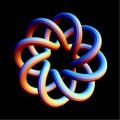
 T(8,3) |
It is well known that the Jones polynomial is related to the Kauffman polynomial via
where [math]\displaystyle{ K }[/math] is some knot or link and where [math]\displaystyle{ c }[/math] is the number of components of [math]\displaystyle{ K }[/math]. Let us verify this fact for the torus knot T(8,3):
In[5]:=
|
K = TorusKnot[8, 3];
|
In[6]:=
|
Simplify[{
  (-1)^(Length[Skeleton[K]]-1)Kauffman[K][-q^(-3/4), q^(1/4)+q^(-1/4)],
  Jones[K][q]
}]
|
Out[6]=
|
  7    9    16   7    9    16
{q  + q  - q  , q  + q  - q  }
|
[Kauffman] ^ L. H. Kauffman, An invariant of regular isotopy, Trans. Amer. Math. Soc. 312 (1990) 417-471.