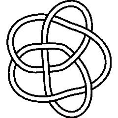
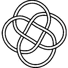
Template:Rolfsen Knot Page: Difference between revisions
No edit summary |
|||
| (62 intermediate revisions by 12 users not shown) | |||
| Line 1: | Line 1: | ||
<span id="top"></span> |
<span id="top"></span> |
||
<noinclude> |
|||
This is the Rolfsen Knot Page master template. For testing purposes, some of the data in it is filled in with data for [[8_17]]. |
|||
</noinclude> |
|||
{{Knot Navigation Links|ext=gif}} |
{{Knot Navigation Links|ext=gif}} |
||
{{TOCright}} |
{{TOCright}} |
||
| Line 8: | Line 11: | ||
See the full [[The Rolfsen Knot Table|Rolfsen Knot Table]]. |
See the full [[The Rolfsen Knot Table|Rolfsen Knot Table]]. |
||
Visit [http://newweb.cecm.sfu.ca/cgi-bin/KnotPlot/KnotServer/kserver?ncomp=1&ncross={{{n}}}&id={{{k}}} {{PAGENAME}}'s page] |
Visit [http://newweb.cecm.sfu.ca/cgi-bin/KnotPlot/KnotServer/kserver?ncomp=1&ncross={{{n}}}&id={{{k}}} {{PAGENAME}}'s page] |
||
at the [http://www.colab.sfu.ca/KnotPlot/KnotServer/ Knot Server] |
|||
([http://www.pims.math.ca/knotplot/ KnotPlot] driven, includes 3D interactive images!) |
|||
Visit [{{{ |
Visit [http://knotilus.math.uwo.ca/draw.php?knot={{urlencode:{{Data:{{PAGENAME}}/Gauss Code}}}} {{PAGENAME}}] at [http://knotilus.math.uwo.ca/ Knotilus]! |
||
Visit [http://www.math.toronto.edu/~drorbn/KAtlas/Knots/{{{n}}}.{{{k}}}.html {{PAGENAME}}'s page] at the original [http://www.math.toronto.edu/~drorbn/KAtlas/index.html Knot Atlas]! |
|||
|- |
|- |
||
| |
|{{floating edit link|{{PAGENAME}} Quick Notes}} |
||
{{#ifexist:{{PAGENAME}} Quick Notes|{{:{{PAGENAME}} Quick Notes}}|}} |
|||
|} |
|} |
||
{{edit link|{{PAGENAME}} Further Notes and Views}} |
{{floating edit link|{{PAGENAME}} Further Notes and Views}} |
||
{{#ifexist:{{PAGENAME}} Further Notes and Views|{{:{{PAGENAME}} Further Notes and Views}}|}} |
|||
<div style="border: solid pink 1px"> |
<div style="border: solid pink 1px"> |
||
{{Knot Presentations}} |
{{Knot Presentations}} |
||
<br style="clear:both" /> |
|||
{| |
|||
{| align=center width=99% |
|||
|- valign=top |
|- align=center valign=top |
||
|'''[[Braid Representatives|Minimum Braid Representative]]''' |
|width=33%|'''[[Braid Representatives|Minimum Braid Representative]]''' |
||
| ⚫ | |||
| ⚫ | |||
|width=33%|'''[[Arc Presentations|An Arc Presentation]]''' |
|||
[[Invariants from Braid Theory|Braid index]] is {{{braid_index}}}) |
|||
| ⚫ | |||
|style="padding-left: 1em;" | {{{braid_table}}} |
|||
|{{Data:{{PAGENAME}}/BraidPlot}}<br>[[Invariants from Braid Theory|Length]] is {{Data:{{PAGENAME}}/MinimalBraidLength}}, width is {{Data:{{PAGENAME}}/MinimalBraidWidth}}, |
|||
| ⚫ | |||
| ⚫ | |||
| ⚫ | |||
| |
|[[Image:{{PAGENAME}}_ML.gif]] |
||
|[[Image:{{PAGENAME}}_AP.gif]]<br>{{Data:{{PAGENAME}}/Arc_Presentation}} |
|||
|} |
|} |
||
{{edit link|Notes on presentations of {{PAGENAME}}}} |
{{edit link|Notes on presentations of {{PAGENAME}}}} |
||
{{#ifexist:Notes on presentations of {{PAGENAME}}|{{:Notes on presentations of {{PAGENAME}}}}|}} |
|||
{{Rolfsen Knot Presentations Computer Talk}} |
|||
</div> |
</div> |
||
| Line 42: | Line 47: | ||
{{4D Invariants}} |
{{4D Invariants}} |
||
{{Polynomial Invariants}} |
{{Polynomial Invariants}} |
||
{{Similar Knots| |
{{Similar Knots| |
||
same_alexander = {{{same_alexander}}} | |
same_alexander = {{{same_alexander}}} | |
||
| Line 48: | Line 52: | ||
{{Vassiliev Invariants}} |
{{Vassiliev Invariants}} |
||
{{Khovanov Homology |
{{Khovanov Homology}} |
||
{{Coloured Jones| |
{{Coloured Jones| |
||
| Line 57: | Line 61: | ||
J6 = {{{coloured_jones_6}}} | |
J6 = {{{coloured_jones_6}}} | |
||
J7 = {{{coloured_jones_7}}} }} |
J7 = {{{coloured_jones_7}}} }} |
||
| ⚫ | |||
| ⚫ | |||
<div style="border: solid pink 1px"> |
<div style="border: solid pink 1px"> |
||
| Line 74: | Line 77: | ||
|} |
|} |
||
| ⚫ | |||
</div> |
</div> |
||
| ⚫ | |||
Latest revision as of 00:06, 3 July 2015
This is the Rolfsen Knot Page master template. For testing purposes, some of the data in it is filled in with data for 8_17.
|
|
|
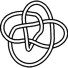 (KnotPlot image) |
See the full Rolfsen Knot Table. Visit Rolfsen Knot Page's page at the Knot Server (KnotPlot driven, includes 3D interactive images!) Visit Rolfsen Knot Page at Knotilus! |
Knot presentations
| Minimum Braid Representative | A Morse Link Presentation | An Arc Presentation | |||
Length is 8, width is 3, Braid index is 3 |
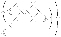
|
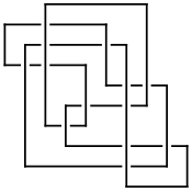 [{7, 10}, {9, 2}, {10, 4}, {3, 5}, {4, 8}, {6, 9}, {5, 1}, {2, 7}, {1, 6}, {8, 3}] |
[edit Notes on presentations of Rolfsen Knot Page]
KnotTheory`. Your input (in red) is realistic; all else should have the same content as in a real mathematica session, but with different formatting.
(The path below may be different on your system, and possibly also the KnotTheory` date)
In[1]:=
|
AppendTo[$Path, "C:/drorbn/projects/KAtlas/"];
<< KnotTheory`
|
Loading KnotTheory` version of May 31, 2006, 14:15:20.091.
|
In[3]:=
|
K = Knot["Rolfsen Knot Page"];
|
In[4]:=
|
PD[K]
|
KnotTheory::loading: Loading precomputed data in PD4Knots`.
|
Out[4]=
|
Data:Rolfsen Knot Page/PD Presentation |
In[5]:=
|
GaussCode[K]
|
Out[5]=
|
Data:Rolfsen Knot Page/Gauss Code |
In[6]:=
|
DTCode[K]
|
Out[6]=
|
Data:Rolfsen Knot Page/DT Code |
(The path below may be different on your system)
In[7]:=
|
AppendTo[$Path, "C:/bin/LinKnot/"];
|
In[8]:=
|
ConwayNotation[K]
|
Out[8]=
|
Data:Rolfsen Knot Page/Conway Notation |
In[9]:=
|
br = BR[K]
|
KnotTheory::credits: The minimum braids representing the knots with up to 10 crossings were provided by Thomas Gittings. See arXiv:math.GT/0401051.
|
Out[9]=
|
Data:Rolfsen Knot Page/BraidWord |
In[10]:=
|
{First[br], Crossings[br], BraidIndex[K]}
|
KnotTheory::credits: The braid index data known to KnotTheory` is taken from Charles Livingston's http://www.indiana.edu/~knotinfo/.
|
KnotTheory::loading: Loading precomputed data in IndianaData`.
|
Out[10]=
|
{ 3, 8, 3 } |
In[11]:=
|
Show[BraidPlot[br]]
|
Out[11]=
|
-Graphics- |
In[12]:=
|
Show[DrawMorseLink[K]]
|
KnotTheory::credits: "MorseLink was added to KnotTheory` by Siddarth Sankaran at the University of Toronto in the summer of 2005."
|
KnotTheory::credits: "DrawMorseLink was written by Siddarth Sankaran at the University of Toronto in the summer of 2005."
|

|
Out[12]=
|
-Graphics- |
In[13]:=
|
ap = ArcPresentation[K]
|
Out[13]=
|
ArcPresentation[{7, 10}, {9, 2}, {10, 4}, {3, 5}, {4, 8}, {6, 9}, {5, 1}, {2, 7}, {1, 6}, {8, 3}] |
In[14]:=
|
Draw[ap]
|

|
Out[14]=
|
-Graphics- |
Three dimensional invariants
|
[edit Notes for Rolfsen Knot Page's three dimensional invariants] |
Four dimensional invariants
|
[edit Notes for Rolfsen Knot Page's four dimensional invariants] |
Polynomial invariants
KnotTheory`, as shown in the (simulated) Mathematica session below. Your input (in red) is realistic; all else should have the same content as in a real mathematica session, but with different formatting. This Mathematica session is also available (albeit only for the knot 5_2) as the notebook PolynomialInvariantsSession.nb.
(The path below may be different on your system, and possibly also the KnotTheory` date)
In[1]:=
|
AppendTo[$Path, "C:/drorbn/projects/KAtlas/"];
<< KnotTheory`
|
Loading KnotTheory` version of August 31, 2006, 11:25:27.5625.
|
In[3]:=
|
K = Knot["Rolfsen Knot Page"];
|
In[4]:=
|
Alexander[K][t]
|
KnotTheory::loading: Loading precomputed data in PD4Knots`.
|
Out[4]=
|
Data:Rolfsen Knot Page/Alexander Polynomial |
In[5]:=
|
Conway[K][z]
|
Out[5]=
|
Data:Rolfsen Knot Page/Conway Polynomial |
In[6]:=
|
Alexander[K, 2][t]
|
KnotTheory::credits: The program Alexander[K, r] to compute Alexander ideals was written by Jana Archibald at the University of Toronto in the summer of 2005.
|
Out[6]=
|
Data:Rolfsen Knot Page/2nd AlexanderIdeal |
In[7]:=
|
{KnotDet[K], KnotSignature[K]}
|
Out[7]=
|
{ Data:Rolfsen Knot Page/Determinant, Data:Rolfsen Knot Page/Signature } |
In[8]:=
|
Jones[K][q]
|
KnotTheory::loading: Loading precomputed data in Jones4Knots`.
|
Out[8]=
|
Data:Rolfsen Knot Page/Jones Polynomial |
In[9]:=
|
HOMFLYPT[K][a, z]
|
KnotTheory::credits: The HOMFLYPT program was written by Scott Morrison.
|
Out[9]=
|
Data:Rolfsen Knot Page/HOMFLYPT Polynomial |
In[10]:=
|
Kauffman[K][a, z]
|
KnotTheory::loading: Loading precomputed data in Kauffman4Knots`.
|
Out[10]=
|
Data:Rolfsen Knot Page/Kauffman Polynomial |
"Similar" Knots (within the Atlas)
Same Alexander/Conway Polynomial: {{{{same_alexander}}}}
Same Jones Polynomial (up to mirroring, ): {{{{same_jones}}}}
KnotTheory`. Your input (in red) is realistic; all else should have the same content as in a real mathematica session, but with different formatting.
(The path below may be different on your system, and possibly also the KnotTheory` date)
In[1]:=
|
AppendTo[$Path, "C:/drorbn/projects/KAtlas/"];
<< KnotTheory`
|
Loading KnotTheory` version of May 31, 2006, 14:15:20.091.
|
In[3]:=
|
K = Knot["Rolfsen Knot Page"];
|
In[4]:=
|
{A = Alexander[K][t], J = Jones[K][q]}
|
KnotTheory::loading: Loading precomputed data in PD4Knots`.
|
KnotTheory::loading: Loading precomputed data in Jones4Knots`.
|
Out[4]=
|
{ Data:Rolfsen Knot Page/Alexander Polynomial, Data:Rolfsen Knot Page/Jones Polynomial } |
In[5]:=
|
DeleteCases[Select[AllKnots[], (A === Alexander[#][t]) &], K]
|
KnotTheory::loading: Loading precomputed data in DTCode4KnotsTo11`.
|
KnotTheory::credits: The GaussCode to PD conversion was written by Siddarth Sankaran at the University of Toronto in the summer of 2005.
|
Out[5]=
|
{{{{same_alexander}}}} |
In[6]:=
|
DeleteCases[
  Select[
    AllKnots[],
    (J === Jones[#][q] || (J /. q -> 1/q) === Jones[#][q]) &
    ],
  K
  ]
|
KnotTheory::loading: Loading precomputed data in Jones4Knots11`.
|
Out[6]=
|
{{{{same_jones}}}} |
Vassiliev invariants
| V2 and V3: | (Data:Rolfsen Knot Page/V 2, Data:Rolfsen Knot Page/V 3) |
| V2,1 through V6,9: |
V2,1 through V6,9 were provided by Petr Dunin-Barkowski <barkovs@itep.ru>, Andrey Smirnov <asmirnov@itep.ru>, and Alexei Sleptsov <sleptsov@itep.ru> and uploaded on October 2010 by User:Drorbn. Note that they are normalized differently than V2 and V3.
Khovanov Homology
| The coefficients of the monomials are shown, along with their alternating sums (fixed , alternation over ). The squares with yellow highlighting are those on the "critical diagonals", where or , where Data:Rolfsen Knot Page/Signature is the signature of Rolfsen Knot Page. Nonzero entries off the critical diagonals (if any exist) are highlighted in red. | Data:Rolfsen Knot Page/KhovanovTable |
| Integral Khovanov Homology
(db, data source) |
Data:Rolfsen Knot Page/Integral Khovanov Homology |
The Coloured Jones Polynomials
| 2 | {{{coloured_jones_2}}} |
| 3 | {{{coloured_jones_3}}} |
| 4 | {{{coloured_jones_4}}} |
| 5 | {{{coloured_jones_5}}} |
| 6 | {{{coloured_jones_6}}} |
| 7 | {{{coloured_jones_7}}} |
Computer Talk
Much of the above data can be recomputed by Mathematica using the package KnotTheory`. See A Sample KnotTheory` Session, or any of the Computer Talk sections above.
Modifying This Page
| Read me first: Modifying Knot Pages
See/edit the Rolfsen Knot Page master template (intermediate). See/edit the Rolfsen_Splice_Base (expert). Back to the top. |
|
