8 16
|
|
|
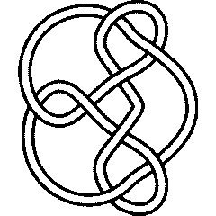
 (KnotPlot image) |
See the full Rolfsen Knot Table. Visit 8 16's page at the Knot Server (KnotPlot driven, includes 3D interactive images!) |

Knot presentations
| Planar diagram presentation | X6271 X14,6,15,5 X16,11,1,12 X12,7,13,8 X8394 X4,9,5,10 X10,15,11,16 X2,14,3,13 |
| Gauss code | 1, -8, 5, -6, 2, -1, 4, -5, 6, -7, 3, -4, 8, -2, 7, -3 |
| Dowker-Thistlethwaite code | 6 8 14 12 4 16 2 10 |
| Conway Notation | [.2.20] |
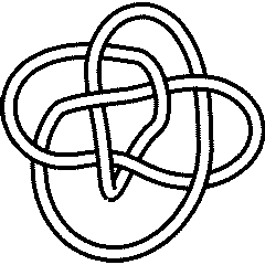
| Minimum Braid Representative | A Morse Link Presentation | An Arc Presentation | |||
Length is 8, width is 3, Braid index is 3 |

|
 [{3, 10}, {2, 6}, {8, 11}, {9, 7}, {4, 8}, {6, 9}, {5, 3}, {10, 4}, {1, 5}, {11, 2}, {7, 1}] |
[edit Notes on presentations of 8 16]


KnotTheory`. Your input (in red) is realistic; all else should have the same content as in a real mathematica session, but with different formatting.
(The path below may be different on your system, and possibly also the KnotTheory` date)
In[1]:=
|
AppendTo[$Path, "C:/drorbn/projects/KAtlas/"];
<< KnotTheory`
|
Loading KnotTheory` version of May 31, 2006, 14:15:20.091.
|
In[3]:=
|
K = Knot["8 16"];
|
In[4]:=
|
PD[K]
|
KnotTheory::loading: Loading precomputed data in PD4Knots`.
|
Out[4]=
|
X6271 X14,6,15,5 X16,11,1,12 X12,7,13,8 X8394 X4,9,5,10 X10,15,11,16 X2,14,3,13 |
In[5]:=
|
GaussCode[K]
|
Out[5]=
|
1, -8, 5, -6, 2, -1, 4, -5, 6, -7, 3, -4, 8, -2, 7, -3 |
In[6]:=
|
DTCode[K]
|
Out[6]=
|
6 8 14 12 4 16 2 10 |
(The path below may be different on your system)
In[7]:=
|
AppendTo[$Path, "C:/bin/LinKnot/"];
|
In[8]:=
|
ConwayNotation[K]
|
Out[8]=
|
[.2.20] |
In[9]:=
|
br = BR[K]
|
KnotTheory::credits: The minimum braids representing the knots with up to 10 crossings were provided by Thomas Gittings. See arXiv:math.GT/0401051.
|
Out[9]=
|
[math]\displaystyle{ \textrm{BR}(3,\{-1,-1,2,-1,-1,2,-1,2\}) }[/math] |
In[10]:=
|
{First[br], Crossings[br], BraidIndex[K]}
|
KnotTheory::credits: The braid index data known to KnotTheory` is taken from Charles Livingston's http://www.indiana.edu/~knotinfo/.
|
KnotTheory::loading: Loading precomputed data in IndianaData`.
|
Out[10]=
|
{ 3, 8, 3 } |
In[11]:=
|
Show[BraidPlot[br]]
|
Out[11]=
|
-Graphics- |
In[12]:=
|
Show[DrawMorseLink[K]]
|
KnotTheory::credits: "MorseLink was added to KnotTheory` by Siddarth Sankaran at the University of Toronto in the summer of 2005."
|
KnotTheory::credits: "DrawMorseLink was written by Siddarth Sankaran at the University of Toronto in the summer of 2005."
|
|
|
Out[12]=
|
-Graphics- |
In[13]:=
|
ap = ArcPresentation[K]
|
Out[13]=
|
ArcPresentation[{3, 10}, {2, 6}, {8, 11}, {9, 7}, {4, 8}, {6, 9}, {5, 3}, {10, 4}, {1, 5}, {11, 2}, {7, 1}] |
In[14]:=
|
Draw[ap]
|
|
|
Out[14]=
|
-Graphics- |
Three dimensional invariants
|
Four dimensional invariants
|
Polynomial invariants
| Alexander polynomial | [math]\displaystyle{ t^3-4 t^2+8 t-9+8 t^{-1} -4 t^{-2} + t^{-3} }[/math] |
| Conway polynomial | [math]\displaystyle{ z^6+2 z^4+z^2+1 }[/math] |
| 2nd Alexander ideal (db, data sources) | [math]\displaystyle{ \{1\} }[/math] |
| Determinant and Signature | { 35, -2 } |
| Jones polynomial | [math]\displaystyle{ -q^2+3 q-4+6 q^{-1} -6 q^{-2} +6 q^{-3} -5 q^{-4} +3 q^{-5} - q^{-6} }[/math] |
| HOMFLY-PT polynomial (db, data sources) | [math]\displaystyle{ a^2 z^6-a^4 z^4+4 a^2 z^4-z^4-2 a^4 z^2+5 a^2 z^2-2 z^2-a^4+2 a^2 }[/math] |
| Kauffman polynomial (db, data sources) | [math]\displaystyle{ z^3 a^7+3 z^4 a^6-z^2 a^6+5 z^5 a^5-5 z^3 a^5+2 z a^5+5 z^6 a^4-7 z^4 a^4+4 z^2 a^4-a^4+2 z^7 a^3+3 z^5 a^3-10 z^3 a^3+4 z a^3+8 z^6 a^2-18 z^4 a^2+10 z^2 a^2-2 a^2+2 z^7 a-z^5 a-6 z^3 a+3 z a+3 z^6-8 z^4+5 z^2+z^5 a^{-1} -2 z^3 a^{-1} +z a^{-1} }[/math] |
| The A2 invariant | [math]\displaystyle{ -q^{18}+q^{16}-q^{14}+q^{10}-q^8+2 q^6-q^4+2 q^2+1+ q^{-4} - q^{-6} }[/math] |
| The G2 invariant | [math]\displaystyle{ q^{100}-2 q^{98}+3 q^{96}-4 q^{94}+2 q^{92}-q^{90}-2 q^{88}+9 q^{86}-12 q^{84}+15 q^{82}-14 q^{80}+7 q^{78}+2 q^{76}-16 q^{74}+28 q^{72}-31 q^{70}+24 q^{68}-10 q^{66}-11 q^{64}+26 q^{62}-30 q^{60}+21 q^{58}-5 q^{56}-15 q^{54}+23 q^{52}-19 q^{50}+2 q^{48}+22 q^{46}-36 q^{44}+36 q^{42}-20 q^{40}-4 q^{38}+30 q^{36}-45 q^{34}+46 q^{32}-33 q^{30}+12 q^{28}+14 q^{26}-32 q^{24}+39 q^{22}-30 q^{20}+14 q^{18}+5 q^{16}-20 q^{14}+24 q^{12}-14 q^{10}-q^8+21 q^6-29 q^4+26 q^2-6-17 q^{-2} +35 q^{-4} -37 q^{-6} +28 q^{-8} -10 q^{-10} -12 q^{-12} +24 q^{-14} -25 q^{-16} +20 q^{-18} -9 q^{-20} -2 q^{-22} +6 q^{-24} -8 q^{-26} +5 q^{-28} -2 q^{-30} + q^{-32} }[/math] |
A1 Invariants.
| Weight | Invariant |
|---|---|
| 1 | [math]\displaystyle{ -q^{13}+2 q^{11}-2 q^9+q^7+2 q- q^{-1} +2 q^{-3} - q^{-5} }[/math] |
| 2 | [math]\displaystyle{ q^{36}-2 q^{34}+5 q^{30}-7 q^{28}-2 q^{26}+11 q^{24}-6 q^{22}-5 q^{20}+8 q^{18}-q^{16}-5 q^{14}+q^{12}+5 q^{10}-2 q^8-5 q^6+7 q^4+2 q^2-9+6 q^{-2} +6 q^{-4} -8 q^{-6} + q^{-8} +6 q^{-10} -3 q^{-12} -2 q^{-14} + q^{-16} }[/math] |
| 3 | [math]\displaystyle{ -q^{69}+2 q^{67}-3 q^{63}+q^{61}+6 q^{59}-16 q^{55}+26 q^{51}+6 q^{49}-33 q^{47}-19 q^{45}+35 q^{43}+28 q^{41}-30 q^{39}-32 q^{37}+19 q^{35}+34 q^{33}-5 q^{31}-28 q^{29}-8 q^{27}+20 q^{25}+15 q^{23}-12 q^{21}-24 q^{19}+5 q^{17}+29 q^{15}+2 q^{13}-32 q^{11}-6 q^9+34 q^7+16 q^5-32 q^3-25 q+28 q^{-1} +31 q^{-3} -16 q^{-5} -35 q^{-7} +5 q^{-9} +33 q^{-11} +7 q^{-13} -24 q^{-15} -13 q^{-17} +12 q^{-19} +15 q^{-21} -4 q^{-23} -9 q^{-25} -2 q^{-27} +3 q^{-29} +2 q^{-31} - q^{-33} }[/math] |
| 4 | [math]\displaystyle{ q^{112}-2 q^{110}+3 q^{106}-3 q^{104}-4 q^{100}+8 q^{98}+13 q^{96}-16 q^{94}-17 q^{92}-17 q^{90}+36 q^{88}+65 q^{86}-17 q^{84}-75 q^{82}-91 q^{80}+44 q^{78}+160 q^{76}+60 q^{74}-91 q^{72}-198 q^{70}-38 q^{68}+185 q^{66}+163 q^{64}-9 q^{62}-209 q^{60}-134 q^{58}+86 q^{56}+165 q^{54}+89 q^{52}-103 q^{50}-139 q^{48}-29 q^{46}+81 q^{44}+115 q^{42}+12 q^{40}-83 q^{38}-95 q^{36}+3 q^{34}+104 q^{32}+79 q^{30}-45 q^{28}-130 q^{26}-38 q^{24}+99 q^{22}+130 q^{20}-20 q^{18}-163 q^{16}-79 q^{14}+87 q^{12}+180 q^{10}+32 q^8-165 q^6-139 q^4+17 q^2+193+119 q^{-2} -89 q^{-4} -164 q^{-6} -94 q^{-8} +114 q^{-10} +158 q^{-12} +35 q^{-14} -91 q^{-16} -144 q^{-18} -9 q^{-20} +90 q^{-22} +89 q^{-24} +18 q^{-26} -80 q^{-28} -56 q^{-30} -4 q^{-32} +41 q^{-34} +45 q^{-36} -6 q^{-38} -20 q^{-40} -20 q^{-42} -3 q^{-44} +12 q^{-46} +5 q^{-48} +2 q^{-50} -3 q^{-52} -2 q^{-54} + q^{-56} }[/math] |
| 5 | [math]\displaystyle{ -q^{165}+2 q^{163}-3 q^{159}+3 q^{157}+2 q^{155}-2 q^{153}-4 q^{151}-5 q^{149}+16 q^{145}+23 q^{143}-5 q^{141}-47 q^{139}-56 q^{137}+q^{135}+88 q^{133}+133 q^{131}+54 q^{129}-148 q^{127}-270 q^{125}-158 q^{123}+161 q^{121}+436 q^{119}+366 q^{117}-87 q^{115}-593 q^{113}-639 q^{111}-92 q^{109}+642 q^{107}+901 q^{105}+381 q^{103}-545 q^{101}-1081 q^{99}-686 q^{97}+319 q^{95}+1079 q^{93}+926 q^{91}-9 q^{89}-909 q^{87}-1027 q^{85}-283 q^{83}+632 q^{81}+953 q^{79}+492 q^{77}-306 q^{75}-772 q^{73}-588 q^{71}+26 q^{69}+532 q^{67}+573 q^{65}+188 q^{63}-301 q^{61}-515 q^{59}-314 q^{57}+121 q^{55}+446 q^{53}+394 q^{51}-6 q^{49}-406 q^{47}-447 q^{45}-64 q^{43}+409 q^{41}+512 q^{39}+102 q^{37}-444 q^{35}-591 q^{33}-159 q^{31}+485 q^{29}+704 q^{27}+242 q^{25}-502 q^{23}-819 q^{21}-375 q^{19}+450 q^{17}+918 q^{15}+557 q^{13}-325 q^{11}-945 q^9-746 q^7+108 q^5+868 q^3+905 q+178 q^{-1} -685 q^{-3} -956 q^{-5} -454 q^{-7} +383 q^{-9} +878 q^{-11} +668 q^{-13} -46 q^{-15} -663 q^{-17} -733 q^{-19} -257 q^{-21} +361 q^{-23} +642 q^{-25} +439 q^{-27} -53 q^{-29} -440 q^{-31} -465 q^{-33} -162 q^{-35} +194 q^{-37} +354 q^{-39} +259 q^{-41} +4 q^{-43} -201 q^{-45} -224 q^{-47} -99 q^{-49} +52 q^{-51} +134 q^{-53} +115 q^{-55} +21 q^{-57} -52 q^{-59} -68 q^{-61} -39 q^{-63} +26 q^{-67} +28 q^{-69} +8 q^{-71} -5 q^{-73} -8 q^{-75} -5 q^{-77} -2 q^{-79} +3 q^{-81} +2 q^{-83} - q^{-85} }[/math] |
| 6 | [math]\displaystyle{ q^{228}-2 q^{226}+3 q^{222}-3 q^{220}-2 q^{218}+10 q^{214}+q^{212}-8 q^{210}-19 q^{206}-10 q^{204}+21 q^{202}+57 q^{200}+33 q^{198}-31 q^{196}-73 q^{194}-135 q^{192}-75 q^{190}+106 q^{188}+304 q^{186}+281 q^{184}+25 q^{182}-308 q^{180}-659 q^{178}-562 q^{176}+42 q^{174}+883 q^{172}+1266 q^{170}+813 q^{168}-284 q^{166}-1689 q^{164}-2162 q^{162}-1163 q^{160}+975 q^{158}+2814 q^{156}+3056 q^{154}+1343 q^{152}-1837 q^{150}-4170 q^{148}-3998 q^{146}-992 q^{144}+2915 q^{142}+5291 q^{140}+4527 q^{138}+469 q^{136}-4039 q^{134}-6182 q^{132}-4287 q^{130}+289 q^{128}+4762 q^{126}+6374 q^{124}+3726 q^{122}-1108 q^{120}-5157 q^{118}-5719 q^{116}-2863 q^{114}+1612 q^{112}+4916 q^{110}+4828 q^{108}+1928 q^{106}-1918 q^{104}-4121 q^{102}-3794 q^{100}-1232 q^{98}+1821 q^{96}+3366 q^{94}+2838 q^{92}+684 q^{90}-1514 q^{88}-2714 q^{86}-2150 q^{84}-380 q^{82}+1434 q^{80}+2265 q^{78}+1615 q^{76}+57 q^{74}-1565 q^{72}-2025 q^{70}-1146 q^{68}+573 q^{66}+1878 q^{64}+1816 q^{62}+420 q^{60}-1428 q^{58}-2213 q^{56}-1420 q^{54}+671 q^{52}+2378 q^{50}+2383 q^{48}+523 q^{46}-1971 q^{44}-3147 q^{42}-2159 q^{40}+730 q^{38}+3282 q^{36}+3646 q^{34}+1333 q^{32}-2119 q^{30}-4283 q^{28}-3695 q^{26}-273 q^{24}+3444 q^{22}+5009 q^{20}+3166 q^{18}-818 q^{16}-4378 q^{14}-5287 q^{12}-2546 q^{10}+1786 q^8+5046 q^6+5012 q^4+1936 q^2-2346-5245 q^{-2} -4675 q^{-4} -1385 q^{-6} +2685 q^{-8} +4881 q^{-10} +4252 q^{-12} +1110 q^{-14} -2616 q^{-16} -4443 q^{-18} -3709 q^{-20} -876 q^{-22} +2111 q^{-24} +3844 q^{-26} +3229 q^{-28} +835 q^{-30} -1658 q^{-32} -3060 q^{-34} -2633 q^{-36} -978 q^{-38} +1160 q^{-40} +2332 q^{-42} +2106 q^{-44} +900 q^{-46} -623 q^{-48} -1572 q^{-50} -1682 q^{-52} -795 q^{-54} +263 q^{-56} +992 q^{-58} +1131 q^{-60} +696 q^{-62} +16 q^{-64} -602 q^{-66} -702 q^{-68} -501 q^{-70} -106 q^{-72} +244 q^{-74} +412 q^{-76} +347 q^{-78} +92 q^{-80} -78 q^{-82} -190 q^{-84} -179 q^{-86} -97 q^{-88} +17 q^{-90} +83 q^{-92} +70 q^{-94} +51 q^{-96} +7 q^{-98} -20 q^{-100} -34 q^{-102} -16 q^{-104} + q^{-108} +8 q^{-110} +5 q^{-112} +2 q^{-114} -3 q^{-116} -2 q^{-118} + q^{-120} }[/math] |
A2 Invariants.
| Weight | Invariant |
|---|---|
| 1,0 | [math]\displaystyle{ -q^{18}+q^{16}-q^{14}+q^{10}-q^8+2 q^6-q^4+2 q^2+1+ q^{-4} - q^{-6} }[/math] |
| 1,1 | [math]\displaystyle{ q^{52}-4 q^{50}+8 q^{48}-12 q^{46}+22 q^{44}-36 q^{42}+46 q^{40}-62 q^{38}+82 q^{36}-92 q^{34}+96 q^{32}-90 q^{30}+67 q^{28}-34 q^{26}-18 q^{24}+70 q^{22}-120 q^{20}+166 q^{18}-188 q^{16}+200 q^{14}-190 q^{12}+164 q^{10}-124 q^8+70 q^6-20 q^4-28 q^2+76-100 q^{-2} +115 q^{-4} -106 q^{-6} +94 q^{-8} -70 q^{-10} +44 q^{-12} -28 q^{-14} +12 q^{-16} -4 q^{-18} + q^{-20} }[/math] |
| 2,0 | [math]\displaystyle{ q^{46}-q^{44}+2 q^{40}-2 q^{38}-2 q^{36}+3 q^{32}-2 q^{30}-4 q^{28}+4 q^{26}+2 q^{24}-3 q^{22}+4 q^{18}-q^{16}-q^{14}+2 q^{12}-3 q^8-q^6+4 q^4-2 q^2+6 q^{-2} +3 q^{-4} -2 q^{-6} +2 q^{-10} -3 q^{-14} - q^{-16} + q^{-18} }[/math] |
A3 Invariants.
| Weight | Invariant |
|---|---|
| 0,1,0 | [math]\displaystyle{ q^{42}-2 q^{40}-q^{38}+5 q^{36}-3 q^{34}-3 q^{32}+8 q^{30}-4 q^{28}-5 q^{26}+6 q^{24}-4 q^{22}-4 q^{20}+2 q^{18}+q^{16}-q^{12}+5 q^{10}+4 q^8-5 q^6+4 q^4+6 q^2-6+2 q^{-2} +4 q^{-4} -6 q^{-6} +2 q^{-8} + q^{-10} -2 q^{-12} + q^{-14} }[/math] |
| 1,0,0 | [math]\displaystyle{ -q^{23}+q^{21}-2 q^{19}+q^{17}-q^{15}+q^{13}+q^9+q^7+2 q^3+2 q^{-1} - q^{-3} + q^{-5} - q^{-7} }[/math] |
| 1,0,1 | [math]\displaystyle{ q^{68}-4 q^{66}+6 q^{64}-2 q^{62}-7 q^{60}+19 q^{58}-24 q^{56}+9 q^{54}+19 q^{52}-46 q^{50}+54 q^{48}-25 q^{46}-26 q^{44}+76 q^{42}-97 q^{40}+71 q^{38}-10 q^{36}-66 q^{34}+109 q^{32}-114 q^{30}+64 q^{28}-2 q^{26}-41 q^{24}+53 q^{22}-21 q^{20}+3 q^{18}+3 q^{16}+30 q^{14}-75 q^{12}+94 q^{10}-80 q^8+18 q^6+56 q^4-104 q^2+124-82 q^{-2} +36 q^{-4} +28 q^{-6} -59 q^{-8} +60 q^{-10} -43 q^{-12} +10 q^{-14} +7 q^{-16} -14 q^{-18} +10 q^{-20} -4 q^{-22} + q^{-24} }[/math] |
A4 Invariants.
| Weight | Invariant |
|---|---|
| 0,1,0,0 | [math]\displaystyle{ q^{52}-q^{50}-2 q^{48}+3 q^{46}+q^{44}-5 q^{42}+2 q^{40}+6 q^{38}-q^{36}-4 q^{34}+3 q^{32}-9 q^{28}-5 q^{26}+3 q^{24}-4 q^{22}-5 q^{20}+10 q^{18}+4 q^{16}-2 q^{14}+7 q^{12}+9 q^{10}-2 q^8-q^6+5 q^4+2 q^2-5- q^{-2} +3 q^{-4} -2 q^{-6} -2 q^{-8} +2 q^{-10} - q^{-14} + q^{-16} }[/math] |
| 1,0,0,0 | [math]\displaystyle{ -q^{28}+q^{26}-2 q^{24}-q^{18}+q^{16}+2 q^{12}+2 q^8+2 q^4+1+ q^{-2} - q^{-4} + q^{-6} - q^{-8} }[/math] |
B2 Invariants.
| Weight | Invariant |
|---|---|
| 0,1 | [math]\displaystyle{ -q^{42}+2 q^{40}-3 q^{38}+5 q^{36}-7 q^{34}+7 q^{32}-8 q^{30}+6 q^{28}-3 q^{26}+4 q^{22}-6 q^{20}+10 q^{18}-13 q^{16}+14 q^{14}-13 q^{12}+11 q^{10}-8 q^8+5 q^6-2 q^2+6-6 q^{-2} +8 q^{-4} -6 q^{-6} +6 q^{-8} -5 q^{-10} +2 q^{-12} - q^{-14} }[/math] |
| 1,0 | [math]\displaystyle{ q^{68}-2 q^{64}-2 q^{62}+q^{60}+5 q^{58}+2 q^{56}-5 q^{54}-5 q^{52}+2 q^{50}+8 q^{48}+q^{46}-8 q^{44}-4 q^{42}+5 q^{40}+5 q^{38}-4 q^{36}-6 q^{34}+q^{32}+6 q^{30}-6 q^{26}-q^{24}+5 q^{22}+3 q^{20}-3 q^{18}-3 q^{16}+4 q^{14}+5 q^{12}-2 q^{10}-6 q^8+2 q^6+8 q^4+4 q^2-6-6 q^{-2} +4 q^{-4} +8 q^{-6} - q^{-8} -6 q^{-10} -3 q^{-12} +4 q^{-14} +3 q^{-16} -2 q^{-18} -2 q^{-20} + q^{-24} }[/math] |
D4 Invariants.
| Weight | Invariant |
|---|---|
| 1,0,0,0 | [math]\displaystyle{ q^{58}-2 q^{56}+q^{54}-2 q^{52}+5 q^{50}-5 q^{48}+4 q^{46}-5 q^{44}+8 q^{42}-5 q^{40}+3 q^{38}-4 q^{36}+q^{32}-5 q^{30}+2 q^{28}-9 q^{26}+9 q^{24}-9 q^{22}+11 q^{20}-9 q^{18}+12 q^{16}-5 q^{14}+10 q^{12}-4 q^{10}+4 q^8+q^6+2 q^2-4+6 q^{-2} -6 q^{-4} +5 q^{-6} -6 q^{-8} +5 q^{-10} -4 q^{-12} +3 q^{-14} -2 q^{-16} + q^{-18} }[/math] |
G2 Invariants.
| Weight | Invariant |
|---|---|
| 1,0 | [math]\displaystyle{ q^{100}-2 q^{98}+3 q^{96}-4 q^{94}+2 q^{92}-q^{90}-2 q^{88}+9 q^{86}-12 q^{84}+15 q^{82}-14 q^{80}+7 q^{78}+2 q^{76}-16 q^{74}+28 q^{72}-31 q^{70}+24 q^{68}-10 q^{66}-11 q^{64}+26 q^{62}-30 q^{60}+21 q^{58}-5 q^{56}-15 q^{54}+23 q^{52}-19 q^{50}+2 q^{48}+22 q^{46}-36 q^{44}+36 q^{42}-20 q^{40}-4 q^{38}+30 q^{36}-45 q^{34}+46 q^{32}-33 q^{30}+12 q^{28}+14 q^{26}-32 q^{24}+39 q^{22}-30 q^{20}+14 q^{18}+5 q^{16}-20 q^{14}+24 q^{12}-14 q^{10}-q^8+21 q^6-29 q^4+26 q^2-6-17 q^{-2} +35 q^{-4} -37 q^{-6} +28 q^{-8} -10 q^{-10} -12 q^{-12} +24 q^{-14} -25 q^{-16} +20 q^{-18} -9 q^{-20} -2 q^{-22} +6 q^{-24} -8 q^{-26} +5 q^{-28} -2 q^{-30} + q^{-32} }[/math] |
.
KnotTheory`, as shown in the (simulated) Mathematica session below. Your input (in red) is realistic; all else should have the same content as in a real mathematica session, but with different formatting. This Mathematica session is also available (albeit only for the knot 5_2) as the notebook PolynomialInvariantsSession.nb.
(The path below may be different on your system, and possibly also the KnotTheory` date)
In[1]:=
|
AppendTo[$Path, "C:/drorbn/projects/KAtlas/"];
<< KnotTheory`
|
Loading KnotTheory` version of August 31, 2006, 11:25:27.5625.
|
In[3]:=
|
K = Knot["8 16"];
|
In[4]:=
|
Alexander[K][t]
|
KnotTheory::loading: Loading precomputed data in PD4Knots`.
|
Out[4]=
|
[math]\displaystyle{ t^3-4 t^2+8 t-9+8 t^{-1} -4 t^{-2} + t^{-3} }[/math] |
In[5]:=
|
Conway[K][z]
|
Out[5]=
|
[math]\displaystyle{ z^6+2 z^4+z^2+1 }[/math] |
In[6]:=
|
Alexander[K, 2][t]
|
KnotTheory::credits: The program Alexander[K, r] to compute Alexander ideals was written by Jana Archibald at the University of Toronto in the summer of 2005.
|
Out[6]=
|
[math]\displaystyle{ \{1\} }[/math] |
In[7]:=
|
{KnotDet[K], KnotSignature[K]}
|
Out[7]=
|
{ 35, -2 } |
In[8]:=
|
Jones[K][q]
|
KnotTheory::loading: Loading precomputed data in Jones4Knots`.
|
Out[8]=
|
[math]\displaystyle{ -q^2+3 q-4+6 q^{-1} -6 q^{-2} +6 q^{-3} -5 q^{-4} +3 q^{-5} - q^{-6} }[/math] |
In[9]:=
|
HOMFLYPT[K][a, z]
|
KnotTheory::credits: The HOMFLYPT program was written by Scott Morrison.
|
Out[9]=
|
[math]\displaystyle{ a^2 z^6-a^4 z^4+4 a^2 z^4-z^4-2 a^4 z^2+5 a^2 z^2-2 z^2-a^4+2 a^2 }[/math] |
In[10]:=
|
Kauffman[K][a, z]
|
KnotTheory::loading: Loading precomputed data in Kauffman4Knots`.
|
Out[10]=
|
[math]\displaystyle{ z^3 a^7+3 z^4 a^6-z^2 a^6+5 z^5 a^5-5 z^3 a^5+2 z a^5+5 z^6 a^4-7 z^4 a^4+4 z^2 a^4-a^4+2 z^7 a^3+3 z^5 a^3-10 z^3 a^3+4 z a^3+8 z^6 a^2-18 z^4 a^2+10 z^2 a^2-2 a^2+2 z^7 a-z^5 a-6 z^3 a+3 z a+3 z^6-8 z^4+5 z^2+z^5 a^{-1} -2 z^3 a^{-1} +z a^{-1} }[/math] |
"Similar" Knots (within the Atlas)
Same Alexander/Conway Polynomial: {10_156, K11n15, K11n56, K11n58,}
Same Jones Polynomial (up to mirroring, [math]\displaystyle{ q\leftrightarrow q^{-1} }[/math]): {10_156,}
KnotTheory`. Your input (in red) is realistic; all else should have the same content as in a real mathematica session, but with different formatting.
(The path below may be different on your system, and possibly also the KnotTheory` date)
In[1]:=
|
AppendTo[$Path, "C:/drorbn/projects/KAtlas/"];
<< KnotTheory`
|
Loading KnotTheory` version of May 31, 2006, 14:15:20.091.
|
In[3]:=
|
K = Knot["8 16"];
|
In[4]:=
|
{A = Alexander[K][t], J = Jones[K][q]}
|
KnotTheory::loading: Loading precomputed data in PD4Knots`.
|
KnotTheory::loading: Loading precomputed data in Jones4Knots`.
|
Out[4]=
|
{ [math]\displaystyle{ t^3-4 t^2+8 t-9+8 t^{-1} -4 t^{-2} + t^{-3} }[/math], [math]\displaystyle{ -q^2+3 q-4+6 q^{-1} -6 q^{-2} +6 q^{-3} -5 q^{-4} +3 q^{-5} - q^{-6} }[/math] } |
In[5]:=
|
DeleteCases[Select[AllKnots[], (A === Alexander[#][t]) &], K]
|
KnotTheory::loading: Loading precomputed data in DTCode4KnotsTo11`.
|
KnotTheory::credits: The GaussCode to PD conversion was written by Siddarth Sankaran at the University of Toronto in the summer of 2005.
|
Out[5]=
|
{10_156, K11n15, K11n56, K11n58,} |
In[6]:=
|
DeleteCases[
  Select[
    AllKnots[],
    (J === Jones[#][q] || (J /. q -> 1/q) === Jones[#][q]) &
    ],
  K
  ]
|
KnotTheory::loading: Loading precomputed data in Jones4Knots11`.
|
Out[6]=
|
{10_156,} |
Vassiliev invariants
| V2 and V3: | (1, -1) |
| V2,1 through V6,9: |
|
V2,1 through V6,9 were provided by Petr Dunin-Barkowski <barkovs@itep.ru>, Andrey Smirnov <asmirnov@itep.ru>, and Alexei Sleptsov <sleptsov@itep.ru> and uploaded on October 2010 by User:Drorbn. Note that they are normalized differently than V2 and V3.
Khovanov Homology
| The coefficients of the monomials [math]\displaystyle{ t^rq^j }[/math] are shown, along with their alternating sums [math]\displaystyle{ \chi }[/math] (fixed [math]\displaystyle{ j }[/math], alternation over [math]\displaystyle{ r }[/math]). The squares with yellow highlighting are those on the "critical diagonals", where [math]\displaystyle{ j-2r=s+1 }[/math] or [math]\displaystyle{ j-2r=s-1 }[/math], where [math]\displaystyle{ s= }[/math]-2 is the signature of 8 16. Nonzero entries off the critical diagonals (if any exist) are highlighted in red. |
|
| Integral Khovanov Homology
(db, data source) |
|
The Coloured Jones Polynomials
| [math]\displaystyle{ n }[/math] | [math]\displaystyle{ J_n }[/math] |
| 2 | [math]\displaystyle{ q^7-3 q^6-q^5+10 q^4-8 q^3-10 q^2+24 q-8-25 q^{-1} +35 q^{-2} -3 q^{-3} -37 q^{-4} +38 q^{-5} +4 q^{-6} -41 q^{-7} +32 q^{-8} +8 q^{-9} -32 q^{-10} +19 q^{-11} +7 q^{-12} -15 q^{-13} +6 q^{-14} +2 q^{-15} -3 q^{-16} + q^{-17} }[/math] |
| 3 | [math]\displaystyle{ -q^{15}+3 q^{14}+q^{13}-5 q^{12}-8 q^{11}+8 q^{10}+20 q^9-8 q^8-33 q^7-3 q^6+51 q^5+18 q^4-61 q^3-43 q^2+70 q+65-64 q^{-1} -96 q^{-2} +63 q^{-3} +113 q^{-4} -46 q^{-5} -136 q^{-6} +37 q^{-7} +147 q^{-8} -19 q^{-9} -160 q^{-10} +8 q^{-11} +159 q^{-12} +8 q^{-13} -155 q^{-14} -20 q^{-15} +139 q^{-16} +31 q^{-17} -116 q^{-18} -35 q^{-19} +88 q^{-20} +33 q^{-21} -58 q^{-22} -28 q^{-23} +34 q^{-24} +19 q^{-25} -19 q^{-26} -8 q^{-27} +8 q^{-28} +3 q^{-29} -3 q^{-30} -2 q^{-31} +3 q^{-32} - q^{-33} }[/math] |
| 4 | [math]\displaystyle{ q^{26}-3 q^{25}-q^{24}+5 q^{23}+3 q^{22}+8 q^{21}-18 q^{20}-18 q^{19}+5 q^{18}+17 q^{17}+59 q^{16}-22 q^{15}-63 q^{14}-47 q^{13}-7 q^{12}+157 q^{11}+49 q^{10}-62 q^9-146 q^8-142 q^7+210 q^6+175 q^5+61 q^4-190 q^3-350 q^2+140 q+250+269 q^{-1} -116 q^{-2} -526 q^{-3} -16 q^{-4} +224 q^{-5} +466 q^{-6} +32 q^{-7} -619 q^{-8} -182 q^{-9} +140 q^{-10} +609 q^{-11} +182 q^{-12} -650 q^{-13} -319 q^{-14} +48 q^{-15} +694 q^{-16} +306 q^{-17} -625 q^{-18} -420 q^{-19} -50 q^{-20} +706 q^{-21} +401 q^{-22} -522 q^{-23} -454 q^{-24} -160 q^{-25} +596 q^{-26} +437 q^{-27} -330 q^{-28} -378 q^{-29} -239 q^{-30} +376 q^{-31} +362 q^{-32} -130 q^{-33} -206 q^{-34} -217 q^{-35} +153 q^{-36} +202 q^{-37} -23 q^{-38} -55 q^{-39} -117 q^{-40} +37 q^{-41} +67 q^{-42} -7 q^{-43} +3 q^{-44} -35 q^{-45} +8 q^{-46} +14 q^{-47} -7 q^{-48} +4 q^{-49} -6 q^{-50} +3 q^{-51} +2 q^{-52} -3 q^{-53} + q^{-54} }[/math] |
| 5 | [math]\displaystyle{ -q^{40}+3 q^{39}+q^{38}-5 q^{37}-3 q^{36}-3 q^{35}+2 q^{34}+16 q^{33}+21 q^{32}-7 q^{31}-29 q^{30}-42 q^{29}-27 q^{28}+32 q^{27}+94 q^{26}+87 q^{25}-10 q^{24}-124 q^{23}-178 q^{22}-93 q^{21}+117 q^{20}+292 q^{19}+245 q^{18}-29 q^{17}-338 q^{16}-449 q^{15}-186 q^{14}+317 q^{13}+632 q^{12}+463 q^{11}-135 q^{10}-730 q^9-804 q^8-159 q^7+702 q^6+1080 q^5+579 q^4-520 q^3-1299 q^2-996 q+200+1351 q^{-1} +1442 q^{-2} +207 q^{-3} -1336 q^{-4} -1756 q^{-5} -654 q^{-6} +1152 q^{-7} +2062 q^{-8} +1089 q^{-9} -975 q^{-10} -2224 q^{-11} -1479 q^{-12} +708 q^{-13} +2379 q^{-14} +1833 q^{-15} -513 q^{-16} -2443 q^{-17} -2123 q^{-18} +276 q^{-19} +2526 q^{-20} +2379 q^{-21} -103 q^{-22} -2546 q^{-23} -2596 q^{-24} -107 q^{-25} +2567 q^{-26} +2779 q^{-27} +297 q^{-28} -2494 q^{-29} -2921 q^{-30} -542 q^{-31} +2366 q^{-32} +2993 q^{-33} +786 q^{-34} -2109 q^{-35} -2962 q^{-36} -1048 q^{-37} +1752 q^{-38} +2809 q^{-39} +1252 q^{-40} -1311 q^{-41} -2501 q^{-42} -1369 q^{-43} +837 q^{-44} +2065 q^{-45} +1370 q^{-46} -411 q^{-47} -1566 q^{-48} -1216 q^{-49} +77 q^{-50} +1060 q^{-51} +975 q^{-52} +125 q^{-53} -640 q^{-54} -696 q^{-55} -182 q^{-56} +326 q^{-57} +428 q^{-58} +171 q^{-59} -134 q^{-60} -243 q^{-61} -112 q^{-62} +51 q^{-63} +109 q^{-64} +59 q^{-65} -12 q^{-66} -41 q^{-67} -33 q^{-68} +6 q^{-69} +22 q^{-70} +2 q^{-71} -3 q^{-72} + q^{-73} -5 q^{-74} - q^{-75} +6 q^{-76} -3 q^{-77} -2 q^{-78} +3 q^{-79} - q^{-80} }[/math] |
| 6 | [math]\displaystyle{ q^{57}-3 q^{56}-q^{55}+5 q^{54}+3 q^{53}+3 q^{52}-7 q^{51}-19 q^{49}-19 q^{48}+19 q^{47}+30 q^{46}+47 q^{45}+12 q^{44}+13 q^{43}-85 q^{42}-133 q^{41}-63 q^{40}+19 q^{39}+159 q^{38}+182 q^{37}+268 q^{36}-20 q^{35}-301 q^{34}-413 q^{33}-376 q^{32}-42 q^{31}+282 q^{30}+886 q^{29}+660 q^{28}+134 q^{27}-552 q^{26}-1105 q^{25}-1100 q^{24}-605 q^{23}+996 q^{22}+1609 q^{21}+1657 q^{20}+654 q^{19}-879 q^{18}-2272 q^{17}-2743 q^{16}-659 q^{15}+1182 q^{14}+3059 q^{13}+3147 q^{12}+1515 q^{11}-1657 q^{10}-4476 q^9-3646 q^8-1651 q^7+2325 q^6+4974 q^5+5241 q^4+1485 q^3-3847 q^2-5842 q-5721-965 q^{-1} +4404 q^{-2} +8140 q^{-3} +5767 q^{-4} -771 q^{-5} -5808 q^{-6} -8981 q^{-7} -5297 q^{-8} +1663 q^{-9} +9049 q^{-10} +9327 q^{-11} +3213 q^{-12} -3965 q^{-13} -10546 q^{-14} -9014 q^{-15} -1759 q^{-16} +8461 q^{-17} +11491 q^{-18} +6665 q^{-19} -1652 q^{-20} -10910 q^{-21} -11566 q^{-22} -4648 q^{-23} +7473 q^{-24} +12667 q^{-25} +9159 q^{-26} +208 q^{-27} -10915 q^{-28} -13273 q^{-29} -6739 q^{-30} +6680 q^{-31} +13452 q^{-32} +11007 q^{-33} +1604 q^{-34} -10853 q^{-35} -14578 q^{-36} -8458 q^{-37} +5801 q^{-38} +13912 q^{-39} +12629 q^{-40} +3162 q^{-41} -10203 q^{-42} -15409 q^{-43} -10272 q^{-44} +4031 q^{-45} +13348 q^{-46} +13829 q^{-47} +5360 q^{-48} -8049 q^{-49} -14881 q^{-50} -11817 q^{-51} +978 q^{-52} +10786 q^{-53} +13502 q^{-54} +7563 q^{-55} -4203 q^{-56} -11981 q^{-57} -11729 q^{-58} -2326 q^{-59} +6311 q^{-60} +10646 q^{-61} +8125 q^{-62} -154 q^{-63} -7147 q^{-64} -9081 q^{-65} -3938 q^{-66} +1838 q^{-67} +6070 q^{-68} +6230 q^{-69} +1989 q^{-70} -2639 q^{-71} -5023 q^{-72} -3174 q^{-73} -538 q^{-74} +2163 q^{-75} +3224 q^{-76} +1817 q^{-77} -306 q^{-78} -1843 q^{-79} -1461 q^{-80} -780 q^{-81} +324 q^{-82} +1086 q^{-83} +818 q^{-84} +167 q^{-85} -438 q^{-86} -364 q^{-87} -327 q^{-88} -59 q^{-89} +245 q^{-90} +214 q^{-91} +70 q^{-92} -87 q^{-93} -31 q^{-94} -71 q^{-95} -36 q^{-96} +47 q^{-97} +33 q^{-98} +10 q^{-99} -25 q^{-100} +11 q^{-101} -7 q^{-102} -12 q^{-103} +11 q^{-104} +2 q^{-105} + q^{-106} -6 q^{-107} +3 q^{-108} +2 q^{-109} -3 q^{-110} + q^{-111} }[/math] |
| 7 | [math]\displaystyle{ -q^{77}+3 q^{76}+q^{75}-5 q^{74}-3 q^{73}-3 q^{72}+7 q^{71}+5 q^{70}+3 q^{69}+17 q^{68}+7 q^{67}-20 q^{66}-35 q^{65}-50 q^{64}-13 q^{63}+24 q^{62}+39 q^{61}+119 q^{60}+117 q^{59}+50 q^{58}-63 q^{57}-236 q^{56}-265 q^{55}-206 q^{54}-102 q^{53}+231 q^{52}+496 q^{51}+605 q^{50}+507 q^{49}-59 q^{48}-577 q^{47}-990 q^{46}-1207 q^{45}-684 q^{44}+181 q^{43}+1236 q^{42}+2115 q^{41}+1858 q^{40}+879 q^{39}-694 q^{38}-2595 q^{37}-3326 q^{36}-2899 q^{35}-954 q^{34}+2197 q^{33}+4399 q^{32}+5232 q^{31}+3816 q^{30}-72 q^{29}-4116 q^{28}-7274 q^{27}-7578 q^{26}-3711 q^{25}+1847 q^{24}+7752 q^{23}+10998 q^{22}+8840 q^{21}+2904 q^{20}-5758 q^{19}-13028 q^{18}-14181 q^{17}-9460 q^{16}+851 q^{15}+12286 q^{14}+18243 q^{13}+16969 q^{12}+6719 q^{11}-8340 q^{10}-19818 q^9-23784 q^8-15878 q^7+1107 q^6+18085 q^5+28705 q^4+25303 q^3+8356 q^2-12909 q-30600-33687 q^{-1} -19117 q^{-2} +4988 q^{-3} +29521 q^{-4} +39865 q^{-5} +29561 q^{-6} +4823 q^{-7} -25363 q^{-8} -43600 q^{-9} -39112 q^{-10} -15197 q^{-11} +19379 q^{-12} +44807 q^{-13} +46617 q^{-14} +25329 q^{-15} -11993 q^{-16} -44047 q^{-17} -52503 q^{-18} -34421 q^{-19} +4638 q^{-20} +41971 q^{-21} +56398 q^{-22} +42097 q^{-23} +2550 q^{-24} -39239 q^{-25} -59199 q^{-26} -48383 q^{-27} -8627 q^{-28} +36527 q^{-29} +60871 q^{-30} +53343 q^{-31} +13846 q^{-32} -34098 q^{-33} -62288 q^{-34} -57325 q^{-35} -17878 q^{-36} +32218 q^{-37} +63392 q^{-38} +60622 q^{-39} +21301 q^{-40} -30840 q^{-41} -64672 q^{-42} -63577 q^{-43} -24173 q^{-44} +29684 q^{-45} +65879 q^{-46} +66514 q^{-47} +27181 q^{-48} -28413 q^{-49} -67044 q^{-50} -69481 q^{-51} -30530 q^{-52} +26397 q^{-53} +67545 q^{-54} +72462 q^{-55} +34715 q^{-56} -23142 q^{-57} -66976 q^{-58} -75019 q^{-59} -39541 q^{-60} +18181 q^{-61} +64426 q^{-62} +76462 q^{-63} +44850 q^{-64} -11370 q^{-65} -59471 q^{-66} -75993 q^{-67} -49674 q^{-68} +3119 q^{-69} +51715 q^{-70} +72699 q^{-71} +53060 q^{-72} +5813 q^{-73} -41513 q^{-74} -66212 q^{-75} -53989 q^{-76} -14044 q^{-77} +29826 q^{-78} +56667 q^{-79} +51610 q^{-80} +20314 q^{-81} -17896 q^{-82} -44973 q^{-83} -46094 q^{-84} -23700 q^{-85} +7529 q^{-86} +32625 q^{-87} +37962 q^{-88} +23751 q^{-89} +298 q^{-90} -21075 q^{-91} -28709 q^{-92} -21093 q^{-93} -4955 q^{-94} +11823 q^{-95} +19723 q^{-96} +16633 q^{-97} +6638 q^{-98} -5311 q^{-99} -12093 q^{-100} -11767 q^{-101} -6321 q^{-102} +1507 q^{-103} +6674 q^{-104} +7423 q^{-105} +4806 q^{-106} +201 q^{-107} -3153 q^{-108} -4130 q^{-109} -3212 q^{-110} -698 q^{-111} +1305 q^{-112} +2093 q^{-113} +1843 q^{-114} +559 q^{-115} -456 q^{-116} -903 q^{-117} -921 q^{-118} -363 q^{-119} +107 q^{-120} +370 q^{-121} +465 q^{-122} +154 q^{-123} -63 q^{-124} -123 q^{-125} -162 q^{-126} -53 q^{-127} -15 q^{-128} +35 q^{-129} +99 q^{-130} +17 q^{-131} -25 q^{-132} -15 q^{-133} -16 q^{-134} +9 q^{-135} -8 q^{-136} -6 q^{-137} +22 q^{-138} -8 q^{-140} -2 q^{-141} - q^{-142} +6 q^{-143} -3 q^{-144} -2 q^{-145} +3 q^{-146} - q^{-147} }[/math] |
Computer Talk
Much of the above data can be recomputed by Mathematica using the package KnotTheory`. See A Sample KnotTheory` Session, or any of the Computer Talk sections above.
Modifying This Page
| Read me first: Modifying Knot Pages
See/edit the Rolfsen Knot Page master template (intermediate). See/edit the Rolfsen_Splice_Base (expert). Back to the top. |
|