|
|
| Line 1: |
Line 1: |
|
|
<!-- WARNING! WARNING! WARNING! |
|
<!-- This page was generated from the splice template "Torus_Knot_Splice_Template". Please do not edit! --> |
|
<!-- This page was generated from the splice template [[Torus_Knot_Splice_Base]]. Please do not edit! |
| ⚫ |
|
|
|
|
<!-- You probably want to edit the template referred to immediately below. (See [[Category:Knot Page Template]].) |
|
--> |
|
|
|
<!-- This page itself was created by running [[Media:KnotPageSpliceRobot.nb]] on [[Torus_Knot_Splice_Base]]. --> |
|
⚫ |
|
|
|
<!-- --> |
|
|
<!-- WARNING! WARNING! WARNING! |
|
|
<!-- This page was generated from the splice template [[Torus Knot Splice Template]]. Please do not edit! |
|
|
<!-- Almost certainly, you want to edit [[Template:Torus Knot Page]], which actually produces this page. |
|
|
<!-- The text below simply calls [[Template:Torus Knot Page]] setting the values of all the parameters appropriately. |
|
|
<!-- This page itself was created by running [[Media:KnotPageSpliceRobot.nb]] on [[Torus Knot Splice Template]]. --> |
|
|
<!-- --> |
|
{{Torus Knot Page| |
|
{{Torus Knot Page| |
|
m = 5 | |
|
m = 5 | |
Latest revision as of 11:37, 31 August 2005
|
See other torus knots
Visit T(5,2) at Knotilus!
|
| Edit T(5,2) Quick Notes
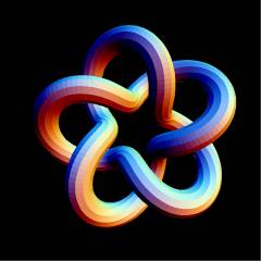
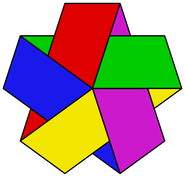
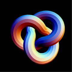
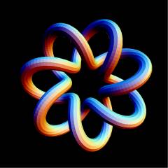
An interlaced pentagram, this is known variously as the "Cinquefoil Knot", after certain herbs and shrubs of the rose family which have 5-lobed leaves and 5-petaled flowers (see e.g. [4]),
as the "Pentafoil Knot" (visit Bert Jagers' pentafoil page),
as the "Double Overhand Knot", as 5_1, or finally as the torus knot T(5,2).
When taken off the post the strangle knot (hitch) of practical knot tying deforms to 5_1
|
Edit T(5,2) Further Notes and Views
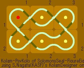 A kolam of a 2x3 dot array |
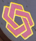
 The VISA Interlink Logo [1] |
|
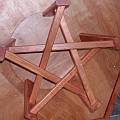 A pentagonal table by Bob Mackay [2] |
 The Utah State Parks logo |
 As impossible object ("Penrose" pentagram) |
 Folded ribbon which is single-sided (more complex version of Möbius Strip). |
|
|
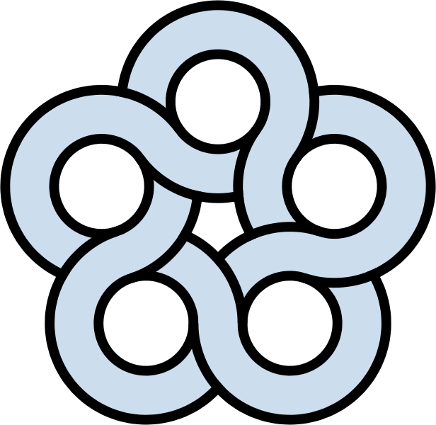 Alternate pentagram of intersecting circles. |
|
 Partial view of US bicentennial logo on a shirt seen in Lisboa [3] |
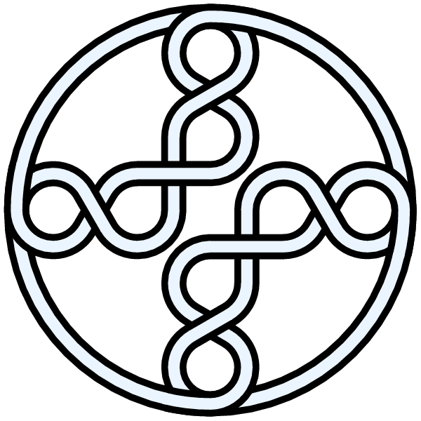 Non-prime knot with two 5_1 configurations on a closed loop. |
|
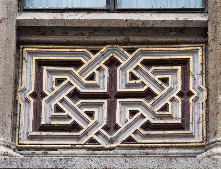 Sum of two 5_1s, Vienna, orthodox church |
This sentence was last edited by Dror.
Sometime later, Scott added this sentence.
Knot presentations
| Planar diagram presentation
|
X3948 X9,5,10,4 X5,1,6,10 X1726 X7382
|
| Gauss code
|
-4, 5, -1, 2, -3, 4, -5, 1, -2, 3
|
| Dowker-Thistlethwaite code
|
6 8 10 2 4
|
Polynomial invariants
Further Quantum Invariants
Computer Talk
The above data is available with the
Mathematica package
KnotTheory`, as shown in the (simulated) Mathematica session below. Your input (in
red) is realistic; all else should have the same content as in a real mathematica session, but with different formatting. This Mathematica session is also available (albeit only for the knot
5_2) as the notebook
PolynomialInvariantsSession.nb.
(The path below may be different on your system, and possibly also the KnotTheory` date)
In[1]:=
|
AppendTo[$Path, "C:/drorbn/projects/KAtlas/"];
<< KnotTheory`
|
In[3]:=
|
K = Knot["T(5,2)"];
|
|
|
KnotTheory::loading: Loading precomputed data in PD4Knots`.
|
Out[4]=
|
[math]\displaystyle{ t^2-t+1- t^{-1} + t^{-2} }[/math]
|
Out[5]=
|
[math]\displaystyle{ z^4+3 z^2+1 }[/math]
|
In[6]:=
|
Alexander[K, 2][t]
|
|
|
KnotTheory::credits: The program Alexander[K, r] to compute Alexander ideals was written by Jana Archibald at the University of Toronto in the summer of 2005.
|
Out[6]=
|
[math]\displaystyle{ \{1\} }[/math]
|
In[7]:=
|
{KnotDet[K], KnotSignature[K]}
|
|
|
KnotTheory::loading: Loading precomputed data in Jones4Knots`.
|
Out[8]=
|
[math]\displaystyle{ -q^7+q^6-q^5+q^4+q^2 }[/math]
|
In[9]:=
|
HOMFLYPT[K][a, z]
|
|
|
KnotTheory::credits: The HOMFLYPT program was written by Scott Morrison.
|
Out[9]=
|
[math]\displaystyle{ z^4 a^{-4} +4 z^2 a^{-4} -z^2 a^{-6} +3 a^{-4} -2 a^{-6} }[/math]
|
In[10]:=
|
Kauffman[K][a, z]
|
|
|
KnotTheory::loading: Loading precomputed data in Kauffman4Knots`.
|
Out[10]=
|
[math]\displaystyle{ z^4 a^{-4} +z^4 a^{-6} +z^3 a^{-5} +z^3 a^{-7} -4 z^2 a^{-4} -3 z^2 a^{-6} +z^2 a^{-8} -2 z a^{-5} -z a^{-7} +z a^{-9} +3 a^{-4} +2 a^{-6} }[/math]
|
"Similar" Knots (within the Atlas)
Same Alexander/Conway Polynomial:
{5_1, 10_132,}
Same Jones Polynomial (up to mirroring, [math]\displaystyle{ q\leftrightarrow q^{-1} }[/math]):
{5_1, 10_132,}
Computer Talk
The above data is available with the
Mathematica package
KnotTheory`. Your input (in
red) is realistic; all else should have the same content as in a real mathematica session, but with different formatting.
(The path below may be different on your system, and possibly also the KnotTheory` date)
In[1]:=
|
AppendTo[$Path, "C:/drorbn/projects/KAtlas/"];
<< KnotTheory`
|
In[3]:=
|
K = Knot["T(5,2)"];
|
In[4]:=
|
{A = Alexander[K][t], J = Jones[K][q]}
|
|
|
KnotTheory::loading: Loading precomputed data in PD4Knots`.
|
|
|
KnotTheory::loading: Loading precomputed data in Jones4Knots`.
|
Out[4]=
|
{ [math]\displaystyle{ t^2-t+1- t^{-1} + t^{-2} }[/math], [math]\displaystyle{ -q^7+q^6-q^5+q^4+q^2 }[/math] }
|
In[5]:=
|
DeleteCases[Select[AllKnots[], (A === Alexander[#][t]) &], K]
|
|
|
KnotTheory::loading: Loading precomputed data in DTCode4KnotsTo11`.
|
|
|
KnotTheory::credits: The GaussCode to PD conversion was written by Siddarth Sankaran at the University of Toronto in the summer of 2005.
|
In[6]:=
|
DeleteCases[
  Select[
    AllKnots[],
    (J === Jones[#][q] || (J /. q -> 1/q) === Jones[#][q]) &
    ],
  K
  ]
|
|
|
KnotTheory::loading: Loading precomputed data in Jones4Knots11`.
|
| V2,1 through V6,9:
|
| V2,1
|
V3,1
|
V4,1
|
V4,2
|
V4,3
|
V5,1
|
V5,2
|
V5,3
|
V5,4
|
V6,1
|
V6,2
|
V6,3
|
V6,4
|
V6,5
|
V6,6
|
V6,7
|
V6,8
|
V6,9
|
| Data:T(5,2)/V 2,1
|
Data:T(5,2)/V 3,1
|
Data:T(5,2)/V 4,1
|
Data:T(5,2)/V 4,2
|
Data:T(5,2)/V 4,3
|
Data:T(5,2)/V 5,1
|
Data:T(5,2)/V 5,2
|
Data:T(5,2)/V 5,3
|
Data:T(5,2)/V 5,4
|
Data:T(5,2)/V 6,1
|
Data:T(5,2)/V 6,2
|
Data:T(5,2)/V 6,3
|
Data:T(5,2)/V 6,4
|
Data:T(5,2)/V 6,5
|
Data:T(5,2)/V 6,6
|
Data:T(5,2)/V 6,7
|
Data:T(5,2)/V 6,8
|
Data:T(5,2)/V 6,9
|
|
V2,1 through V6,9 were provided by Petr Dunin-Barkowski <barkovs@itep.ru>, Andrey Smirnov <asmirnov@itep.ru>, and Alexei Sleptsov <sleptsov@itep.ru> and uploaded on October 2010 by User:Drorbn. Note that they are normalized differently than V2 and V3.
| The coefficients of the monomials [math]\displaystyle{ t^rq^j }[/math] are shown, along with their alternating sums [math]\displaystyle{ \chi }[/math] (fixed [math]\displaystyle{ j }[/math], alternation over [math]\displaystyle{ r }[/math]). The squares with yellow highlighting are those on the "critical diagonals", where [math]\displaystyle{ j-2r=s+1 }[/math] or [math]\displaystyle{ j-2r=s-1 }[/math], where [math]\displaystyle{ s= }[/math]4 is the signature of T(5,2). Nonzero entries off the critical diagonals (if any exist) are highlighted in red.
|
|
|
0 | 1 | 2 | 3 | 4 | 5 | χ |
| 15 | | | | | | 1 | -1 |
| 13 | | | | | | | 0 |
| 11 | | | | 1 | 1 | | 0 |
| 9 | | | | | | | 0 |
| 7 | | | 1 | | | | 1 |
| 5 | 1 | | | | | | 1 |
| 3 | 1 | | | | | | 1 |
|
| Integral Khovanov Homology
(db, data source)
|
|
| [math]\displaystyle{ \dim{\mathcal G}_{2r+i}\operatorname{KH}^r_{\mathbb Z} }[/math]
|
[math]\displaystyle{ i=3 }[/math]
|
[math]\displaystyle{ i=5 }[/math]
|
| [math]\displaystyle{ r=0 }[/math]
|
[math]\displaystyle{ {\mathbb Z} }[/math]
|
[math]\displaystyle{ {\mathbb Z} }[/math]
|
| [math]\displaystyle{ r=1 }[/math]
|
|
|
| [math]\displaystyle{ r=2 }[/math]
|
[math]\displaystyle{ {\mathbb Z} }[/math]
|
|
| [math]\displaystyle{ r=3 }[/math]
|
[math]\displaystyle{ {\mathbb Z}_2 }[/math]
|
[math]\displaystyle{ {\mathbb Z} }[/math]
|
| [math]\displaystyle{ r=4 }[/math]
|
[math]\displaystyle{ {\mathbb Z} }[/math]
|
|
| [math]\displaystyle{ r=5 }[/math]
|
[math]\displaystyle{ {\mathbb Z}_2 }[/math]
|
[math]\displaystyle{ {\mathbb Z} }[/math]
|
|
.jpg)

.png)


