Arc Presentations: Difference between revisions
No edit summary |
mNo edit summary |
||
| (5 intermediate revisions by 2 users not shown) | |||
| Line 1: | Line 1: | ||
{{Manual TOC Sidebar}} |
{{Manual TOC Sidebar}} |
||
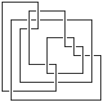
An ''Arc Presentation'' <math>A</math> of a knot <math>K</math> (in "grid form", to be precise) is a planar (toroidal, to be precise) picture of the knot in which all arcs are either horizontal or vertical, in which the vertical arcs are always "above" the horizontal arcs, and in which no two horizontal arcs have the same <math>y</math>-coordinate and no two vertical arcs have the same <math>x</math>-coordinate (read more at [http://www.indiana.edu/~knotinfo/descriptions/arc_index.html]). Without loss of generality, the <math>x</math>-coordinates of the vertical arcs in <math>A</math> are the integers <math>1</math> through <math>n</math> for some <math>n</math>, and the <math>y</math>-coordinates of the horizontal arcs in <math>A</math> are (also!) the integers <math>1</math> through <math>n</math>. |
|||
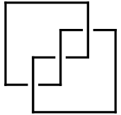
[[Image:3 1 AP.gif|thumb|left|100px|((5,2), (1,3), (2,4), (3,5), (4,1))]] |
|||
Thus for example, on the left is an arc presentation <math>A</math> of the [[3_1|trefoil]] knot. It can be represented numerically by the sequence of ordered pairs shown below it. This sequence reads: the lowest horizontal arc in <math>A</math> connects the 5th vertical arc with the 2nd; the next horizontal arc in <math>A</math> connects the 1st vertical with the 3rd, and so on. In general, an arc presentation involving <math>n</math> horizontal and <math>n</math> vertical arcs will be described in this way by a sequence of <math>n</math> ordered pairs of integers in the range between <math>1</math> and <math>n</math>. |
|||
Arc presentations are used extensively in the computation of [[Heegaard Floer Knot Homology|Heegaard Floer Knot Homologies]]. |
|||
<br clear=left/> |
|||
<code>KnotTheory`</code> knows about arc presentations: |
|||
{{Startup Note}} |
{{Startup Note}} |
||
| Line 7: | Line 17: | ||
n = 1 | |
n = 1 | |
||
in = <nowiki>ArcPresentation</nowiki> | |
in = <nowiki>ArcPresentation</nowiki> | |
||
out= <nowiki>ArcPresentation[{a1,b1}, {a2, b2}, ..., {an,bn}] is an arc presentation of a knot (as often used in the realm of Heegaard-Floer homologies), where |
out= <nowiki>ArcPresentation[{a1,b1}, {a2, b2}, ..., {an,bn}] is an arc presentation of a knot (as often used in the realm of Heegaard-Floer homologies), where the horizontal arc at row i connects column ai to column bi. ArcPresentation[K] returns an arc presentation of the knot K. ArcPresentation[K, Reduce -> r] attemps at most r reduction steps (using a naive reduction algorithm) following a naive creation of some arc presentation for K.</nowiki>}} |
||
<!--END--> |
<!--END--> |
||
{{Knot Image|K11n11|gif}} |
|||
<!--$$ap = ArcPresentation["K11n11"]$$--> |
<!--$$ap = ArcPresentation["K11n11"]$$--> |
||
<!--Robot Land, no human edits to "END"--> |
<!--Robot Land, no human edits to "END"--> |
||
{{InOut| |
|||
n = 2 | |
|||
in = <nowiki>ap = ArcPresentation["K11n11"]</nowiki> | |
|||
out= <nowiki>ArcPresentation[{12, 2}, {1, 10}, {3, 9}, {5, 11}, {9, 12}, {4, 8}, |
|||
{2, 5}, {11, 7}, {8, 6}, {7, 4}, {10, 3}, {6, 1}]</nowiki>}} |
|||
<!--END--> |
<!--END--> |
||
<!--$$Draw[ap]$$--> |
<!--$$Draw[ap]$$--> |
||
<!--Robot Land, no human edits to "END"--> |
<!--Robot Land, no human edits to "END"--> |
||
{{Graphics| |
|||
n = 4 | |
|||
in = <nowiki>Draw[ap]</nowiki> | |
|||
img= Arc_Presentations_Out_3.gif | |
|||
out= <nowiki>-Graphics-</nowiki>}} |
|||
<!--END--> |
<!--END--> |
||
<!--$$ap0 = ArcPresentation["K11n11", Reduce -> 0]$$--> |
<!--$$ap0 = ArcPresentation["K11n11", Reduce -> 0]$$--> |
||
<!--Robot Land, no human edits to "END"--> |
<!--Robot Land, no human edits to "END"--> |
||
{{InOut| |
|||
n = 5 | |
|||
in = <nowiki>ap0 = ArcPresentation["K11n11", Reduce -> 0]</nowiki> | |
|||
out= <nowiki>ArcPresentation[{13, 19}, {20, 23}, {19, 22}, {15, 14}, {14, 2}, |
|||
{1, 13}, {3, 12}, {2, 4}, {16, 18}, {17, 15}, {8, 16}, {12, 17}, |
|||
{5, 7}, {4, 6}, {7, 11}, {6, 8}, {18, 10}, {11, 9}, {10, 21}, |
|||
{9, 20}, {21, 5}, {22, 3}, {23, 1}]</nowiki>}} |
|||
<!--END--> |
<!--END--> |
||
<!--$$?Draw$$--> |
<!--$$?Draw$$--> |
||
<!--Robot Land, no human edits to "END"--> |
<!--Robot Land, no human edits to "END"--> |
||
{{HelpLine| |
|||
n = 6 | |
|||
in = <nowiki>Draw</nowiki> | |
|||
out= <nowiki>Draw[ap] draws the Arc Presentation ap. Draw[ap, OverlayMatrix -> M] overlays the matrix M on top of that draw.</nowiki>}} |
|||
<!--END--> |
<!--END--> |
||
<!--$$Draw[ap0]$$--> |
<!--$$Draw[ap0]$$--> |
||
<!--Robot Land, no human edits to "END"--> |
<!--Robot Land, no human edits to "END"--> |
||
{{Graphics| |
|||
n = 8 | |
|||
in = <nowiki>Draw[ap0]</nowiki> | |
|||
img= Arc_Presentations_Out_7.gif | |
|||
out= <nowiki>-Graphics-</nowiki>}} |
|||
<!--END--> |
<!--END--> |
||
| Line 34: | Line 76: | ||
)$$--> |
)$$--> |
||
<!--Robot Land, no human edits to "END"--> |
<!--Robot Land, no human edits to "END"--> |
||
{{In| |
|||
n = 9 | |
|||
in = <nowiki>Reflect[ap_ArcPresentation] := ArcPresentation @@ ( |
|||
(Last /@ Sort[Reverse /@ Position[ap, #]]) & /@ Range[Length[ap]] |
|||
)</nowiki>}} |
|||
<!--END--> |
<!--END--> |
||
<!--$$Reflect[ap] // Draw$$--> |
<!--$$Reflect[ap] // Draw$$--> |
||
<!--Robot Land, no human edits to "END"--> |
<!--Robot Land, no human edits to "END"--> |
||
{{Graphics| |
|||
n = 11 | |
|||
in = <nowiki>Reflect[ap] // Draw</nowiki> | |
|||
img= Arc_Presentations_Out_10.gif | |
|||
out= <nowiki>-Graphics-</nowiki>}} |
|||
<!--END--> |
<!--END--> |
||
The ''Minesweeper Matrix'' <math>M_A</math> (name not generally accepted) of an arc presentation <math>A</math> of <math>n</math> rows/columns is the <math>n\times n</math> matrix whose <math>(ij)</math> entry is the rotation number of <math>A</math> around a point placed between the <math>i</math> and <math>i+1</math> rows of <math>A</math> and between the <math>j</math> and <math>j+1</math> column of <math>A</math>. Here's a little program to compute the minesweeper matrix of a given arc presentation, along with its output on the arc presentation of [[K11n11]] that we have been studying above: |
|||
<!--$$MinesweeperMatrix[ap_ArcPresentation] := Module[ |
<!--$$MinesweeperMatrix[ap_ArcPresentation] := Module[ |
||
| Line 57: | Line 111: | ||
$$--> |
$$--> |
||
<!--Robot Land, no human edits to "END"--> |
<!--Robot Land, no human edits to "END"--> |
||
{{In| |
|||
n = 12 | |
|||
in = <nowiki>MinesweeperMatrix[ap_ArcPresentation] := Module[ |
|||
{l, CurrentRow, c1, c2, k, s}, |
|||
l = Length[ap]; |
|||
CurrentRow = Table[0, {l}]; |
|||
Table[ |
|||
{c1, c2} = Sort[ap[[k]]]; |
|||
s = Sign[{-1, 1}.ap[[k]]]; |
|||
Do[ |
|||
CurrentRow[[c]] += s, |
|||
{c, c1, c2 - 1} |
|||
]; |
|||
CurrentRow, |
|||
{k, l} |
|||
] |
|||
]; |
|||
</nowiki>}} |
|||
<!--END--> |
<!--END--> |
||
<!--$$Draw[ap, OverlayMatrix -> MinesweeperMatrix[ap]]$$--> |
<!--$$Draw[ap, OverlayMatrix -> MinesweeperMatrix[ap]]$$--> |
||
<!--Robot Land, no human edits to "END"--> |
<!--Robot Land, no human edits to "END"--> |
||
{{Graphics| |
|||
n = 14 | |
|||
in = <nowiki>Draw[ap, OverlayMatrix -> MinesweeperMatrix[ap]]</nowiki> | |
|||
img= Arc_Presentations_Out_13.gif | |
|||
out= <nowiki>-Graphics-</nowiki>}} |
|||
<!--END--> |
<!--END--> |
||
If <math>M_A=(m_{ij})</math>, it is known that the determinant of the matrix <math>(t^{m_{ij}})</math> is the Alexander polynomial of the knot presented by <math>A</math>, up to signs and powers of <math>t</math> and <math>(t-1)</math>. Let us check this in our case: |
|||
<!--$${Det[t^MinesweeperMatrix[ap]], Alexander[ap][t]} // Factor$$--> |
<!--$${Det[t^MinesweeperMatrix[ap]], Alexander[ap][t]} // Factor$$--> |
||
<!--Robot Land, no human edits to "END"--> |
<!--Robot Land, no human edits to "END"--> |
||
{{InOut| |
|||
n = 15 | |
|||
in = <nowiki>{Det[t^MinesweeperMatrix[ap]], Alexander[ap][t]} // Factor</nowiki> | |
|||
out= <nowiki> 11 2 2 3 4 5 6 |
|||
{(-1 + t) t (1 - 5 t + 13 t - 17 t + 13 t - 5 t + t ), |
|||
2 3 4 5 6 |
|||
1 - 5 t + 13 t - 17 t + 13 t - 5 t + t |
|||
-------------------------------------------} |
|||
3 |
|||
t</nowiki>}} |
|||
<!--END--> |
<!--END--> |
||
Latest revision as of 20:55, 5 December 2007
An Arc Presentation [math]\displaystyle{ A }[/math] of a knot [math]\displaystyle{ K }[/math] (in "grid form", to be precise) is a planar (toroidal, to be precise) picture of the knot in which all arcs are either horizontal or vertical, in which the vertical arcs are always "above" the horizontal arcs, and in which no two horizontal arcs have the same [math]\displaystyle{ y }[/math]-coordinate and no two vertical arcs have the same [math]\displaystyle{ x }[/math]-coordinate (read more at [1]). Without loss of generality, the [math]\displaystyle{ x }[/math]-coordinates of the vertical arcs in [math]\displaystyle{ A }[/math] are the integers [math]\displaystyle{ 1 }[/math] through [math]\displaystyle{ n }[/math] for some [math]\displaystyle{ n }[/math], and the [math]\displaystyle{ y }[/math]-coordinates of the horizontal arcs in [math]\displaystyle{ A }[/math] are (also!) the integers [math]\displaystyle{ 1 }[/math] through [math]\displaystyle{ n }[/math].
Thus for example, on the left is an arc presentation [math]\displaystyle{ A }[/math] of the trefoil knot. It can be represented numerically by the sequence of ordered pairs shown below it. This sequence reads: the lowest horizontal arc in [math]\displaystyle{ A }[/math] connects the 5th vertical arc with the 2nd; the next horizontal arc in [math]\displaystyle{ A }[/math] connects the 1st vertical with the 3rd, and so on. In general, an arc presentation involving [math]\displaystyle{ n }[/math] horizontal and [math]\displaystyle{ n }[/math] vertical arcs will be described in this way by a sequence of [math]\displaystyle{ n }[/math] ordered pairs of integers in the range between [math]\displaystyle{ 1 }[/math] and [math]\displaystyle{ n }[/math].
Arc presentations are used extensively in the computation of Heegaard Floer Knot Homologies.
KnotTheory` knows about arc presentations:
(For In[1] see Setup)
| ||||
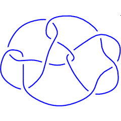 K11n11 |
In[2]:=
|
ap = ArcPresentation["K11n11"]
|
Out[2]=
|
ArcPresentation[{12, 2}, {1, 10}, {3, 9}, {5, 11}, {9, 12}, {4, 8},

  {2, 5}, {11, 7}, {8, 6}, {7, 4}, {10, 3}, {6, 1}]
|
In[4]:=
|
Draw[ap]
|
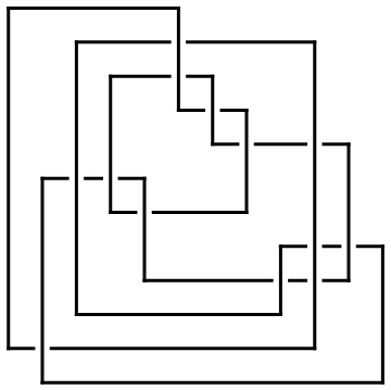
| |
Out[4]=
|
-Graphics-
|
In[5]:=
|
ap0 = ArcPresentation["K11n11", Reduce -> 0]
|
Out[5]=
|
ArcPresentation[{13, 19}, {20, 23}, {19, 22}, {15, 14}, {14, 2},

  {1, 13}, {3, 12}, {2, 4}, {16, 18}, {17, 15}, {8, 16}, {12, 17},

  {5, 7}, {4, 6}, {7, 11}, {6, 8}, {18, 10}, {11, 9}, {10, 21},

  {9, 20}, {21, 5}, {22, 3}, {23, 1}]
|
| ||||
In[8]:=
|
Draw[ap0]
|
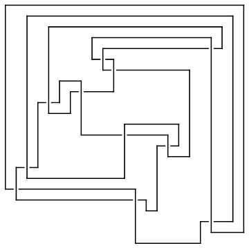
| |
Out[8]=
|
-Graphics-
|
In[9]:=
|
Reflect[ap_ArcPresentation] := ArcPresentation @@ (
  (Last /@ Sort[Reverse /@ Position[ap, #]]) & /@ Range[Length[ap]]
)
|
In[11]:=
|
Reflect[ap] // Draw
|
| |
Out[11]=
|
-Graphics-
|
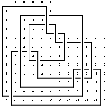
The Minesweeper Matrix [math]\displaystyle{ M_A }[/math] (name not generally accepted) of an arc presentation [math]\displaystyle{ A }[/math] of [math]\displaystyle{ n }[/math] rows/columns is the [math]\displaystyle{ n\times n }[/math] matrix whose [math]\displaystyle{ (ij) }[/math] entry is the rotation number of [math]\displaystyle{ A }[/math] around a point placed between the [math]\displaystyle{ i }[/math] and [math]\displaystyle{ i+1 }[/math] rows of [math]\displaystyle{ A }[/math] and between the [math]\displaystyle{ j }[/math] and [math]\displaystyle{ j+1 }[/math] column of [math]\displaystyle{ A }[/math]. Here's a little program to compute the minesweeper matrix of a given arc presentation, along with its output on the arc presentation of K11n11 that we have been studying above:
In[12]:=
|
MinesweeperMatrix[ap_ArcPresentation] := Module[
  {l, CurrentRow, c1, c2, k, s},
  l = Length[ap];
  CurrentRow = Table[0, {l}];
  Table[
    {c1, c2} = Sort[ap[[k]]];
    s = Sign[{-1, 1}.ap[[k]]];
    Do[
      CurrentRow[[c]] += s,
      {c, c1, c2 - 1}
    ];
    CurrentRow,
    {k, l}
  ]
];
|
In[14]:=
|
Draw[ap, OverlayMatrix -> MinesweeperMatrix[ap]]
|
| |
Out[14]=
|
-Graphics-
|
If [math]\displaystyle{ M_A=(m_{ij}) }[/math], it is known that the determinant of the matrix [math]\displaystyle{ (t^{m_{ij}}) }[/math] is the Alexander polynomial of the knot presented by [math]\displaystyle{ A }[/math], up to signs and powers of [math]\displaystyle{ t }[/math] and [math]\displaystyle{ (t-1) }[/math]. Let us check this in our case:
In[15]:=
|
{Det[t^MinesweeperMatrix[ap]], Alexander[ap][t]} // Factor
|
Out[15]=
|
         11  2                2       3       4      5    6
{(-1 + t)   t  (1 - 5 t + 13 t  - 17 t  + 13 t  - 5 t  + t ),

                2       3       4      5    6
  1 - 5 t + 13 t  - 17 t  + 13 t  - 5 t  + t
  -------------------------------------------}
                       3
                      t
|
