9 16

9_15

9_17

Visit 9 16's page at the Knot Server (KnotPlot driven, includes 3D interactive images!) Visit 9 16's page at Knotilus! Visit 9 16's page at the original Knot Atlas! 9 16 Quick Notes

9 16 Further Notes and Views

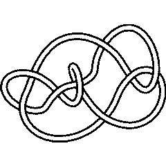
Knot presentations

Planar diagram presentation	X4251 X12,4,13,3 X16,6,17,5 X18,8,1,7 X6,18,7,17 X10,16,11,15 X14,10,15,9 X8,14,9,13 X2,12,3,11
Gauss code	1, -9, 2, -1, 3, -5, 4, -8, 7, -6, 9, -2, 8, -7, 6, -3, 5, -4
Dowker-Thistlethwaite code	4 12 16 18 14 2 8 10 6
Conway Notation	[3,3,2+]

Three dimensional invariants

Symmetry type Reversible Unknotting number 3 3-genus 3 Bridge index 3 Super bridge index [math]\displaystyle{ \{4,7\} }[/math] Nakanishi index 1 Maximal Thurston-Bennequin number [5][-16] Hyperbolic Volume 9.88301 A-Polynomial See Data:9 16/A-polynomial

[edit Notes for 9 16's three dimensional invariants]

Four dimensional invariants

Smooth 4 genus [math]\displaystyle{ 3 }[/math] Topological 4 genus [math]\displaystyle{ 3 }[/math] Concordance genus [math]\displaystyle{ 3 }[/math] Rasmussen s-Invariant -6

[edit Notes for 9 16's four dimensional invariants]

Polynomial invariants

Alexander polynomial	[math]\displaystyle{ 2 t^3-5 t^2+8 t-9+8 t^{-1} -5 t^{-2} +2 t^{-3} }[/math]
Conway polynomial	[math]\displaystyle{ 2 z^6+7 z^4+6 z^2+1 }[/math]
2nd Alexander ideal (db, data sources)	[math]\displaystyle{ \{1\} }[/math]
Determinant and Signature	{ 39, 6 }
Jones polynomial	[math]\displaystyle{ -q^{12}+3 q^{11}-5 q^{10}+6 q^9-7 q^8+6 q^7-5 q^6+4 q^5-q^4+q^3 }[/math]
HOMFLY-PT polynomial (db, data sources)	[math]\displaystyle{ z^6 a^{-6} +z^6 a^{-8} +5 z^4 a^{-6} +3 z^4 a^{-8} -z^4 a^{-10} +8 z^2 a^{-6} -2 z^2 a^{-10} +4 a^{-6} -3 a^{-8} }[/math]
Kauffman polynomial (db, data sources)	[math]\displaystyle{ z^8 a^{-8} +z^8 a^{-10} +z^7 a^{-7} +4 z^7 a^{-9} +3 z^7 a^{-11} +z^6 a^{-6} -z^6 a^{-8} +3 z^6 a^{-10} +5 z^6 a^{-12} -2 z^5 a^{-7} -8 z^5 a^{-9} -z^5 a^{-11} +5 z^5 a^{-13} -5 z^4 a^{-6} -4 z^4 a^{-8} -8 z^4 a^{-10} -6 z^4 a^{-12} +3 z^4 a^{-14} -2 z^3 a^{-7} -z^3 a^{-9} -5 z^3 a^{-11} -5 z^3 a^{-13} +z^3 a^{-15} +8 z^2 a^{-6} +6 z^2 a^{-8} +z^2 a^{-10} +2 z^2 a^{-12} -z^2 a^{-14} +4 z a^{-7} +4 z a^{-9} +2 z a^{-11} +2 z a^{-13} -4 a^{-6} -3 a^{-8} }[/math]
The A2 invariant	[math]\displaystyle{ q^{-10} +3 q^{-14} + q^{-16} +2 q^{-18} + q^{-20} -2 q^{-22} -3 q^{-26} + q^{-34} - q^{-36} }[/math]
The G2 invariant	[math]\displaystyle{ q^{-50} +3 q^{-54} -2 q^{-56} +3 q^{-58} - q^{-60} +8 q^{-64} -11 q^{-66} +16 q^{-68} -11 q^{-70} +6 q^{-72} +11 q^{-74} -21 q^{-76} +32 q^{-78} -26 q^{-80} +18 q^{-82} + q^{-84} -23 q^{-86} +33 q^{-88} -31 q^{-90} +19 q^{-92} -18 q^{-96} +22 q^{-98} -18 q^{-100} +11 q^{-104} -24 q^{-106} +22 q^{-108} -14 q^{-110} -8 q^{-112} +27 q^{-114} -40 q^{-116} +41 q^{-118} -27 q^{-120} +2 q^{-122} +22 q^{-124} -40 q^{-126} +46 q^{-128} -36 q^{-130} +16 q^{-132} +10 q^{-134} -26 q^{-136} +30 q^{-138} -20 q^{-140} +2 q^{-142} +13 q^{-144} -19 q^{-146} +13 q^{-148} - q^{-150} -15 q^{-152} +25 q^{-154} -26 q^{-156} +19 q^{-158} -4 q^{-160} -14 q^{-162} +23 q^{-164} -27 q^{-166} +24 q^{-168} -14 q^{-170} +3 q^{-172} +6 q^{-174} -13 q^{-176} +15 q^{-178} -12 q^{-180} +9 q^{-182} -2 q^{-184} - q^{-186} +2 q^{-188} -4 q^{-190} +3 q^{-192} -2 q^{-194} + q^{-196} }[/math]

Further Quantum Invariants

Further quantum knot invariants for 9_16.

A1 Invariants.

Weight	Invariant
1	[math]\displaystyle{ q^{-5} +3 q^{-9} - q^{-11} + q^{-13} - q^{-15} - q^{-17} + q^{-19} -2 q^{-21} +2 q^{-23} - q^{-25} }[/math]
2	[math]\displaystyle{ q^{-10} +4 q^{-16} + q^{-18} -4 q^{-20} +6 q^{-22} +3 q^{-24} -9 q^{-26} +3 q^{-28} +6 q^{-30} -9 q^{-32} - q^{-34} +6 q^{-36} -4 q^{-38} -4 q^{-40} +3 q^{-42} +3 q^{-44} -4 q^{-46} -2 q^{-48} +9 q^{-50} -3 q^{-52} -8 q^{-54} +9 q^{-56} - q^{-58} -6 q^{-60} +5 q^{-62} -2 q^{-66} + q^{-68} }[/math]
3	[math]\displaystyle{ q^{-15} + q^{-21} +4 q^{-23} + q^{-25} -3 q^{-27} -2 q^{-29} +9 q^{-31} +8 q^{-33} -7 q^{-35} -16 q^{-37} +6 q^{-39} +20 q^{-41} +2 q^{-43} -26 q^{-45} -12 q^{-47} +25 q^{-49} +18 q^{-51} -21 q^{-53} -27 q^{-55} +14 q^{-57} +28 q^{-59} -7 q^{-61} -32 q^{-63} + q^{-65} +27 q^{-67} +8 q^{-69} -26 q^{-71} -9 q^{-73} +21 q^{-75} +16 q^{-77} -13 q^{-79} -19 q^{-81} +3 q^{-83} +21 q^{-85} +8 q^{-87} -22 q^{-89} -19 q^{-91} +18 q^{-93} +29 q^{-95} -14 q^{-97} -32 q^{-99} +8 q^{-101} +31 q^{-103} -3 q^{-105} -23 q^{-107} - q^{-109} +16 q^{-111} -11 q^{-115} +2 q^{-117} +5 q^{-119} -3 q^{-123} +2 q^{-127} - q^{-129} }[/math]
4	[math]\displaystyle{ q^{-20} + q^{-26} + q^{-28} +4 q^{-30} -3 q^{-34} + q^{-38} +13 q^{-40} +6 q^{-42} -8 q^{-44} -15 q^{-46} -15 q^{-48} +22 q^{-50} +30 q^{-52} +11 q^{-54} -26 q^{-56} -60 q^{-58} -4 q^{-60} +44 q^{-62} +65 q^{-64} +16 q^{-66} -86 q^{-68} -68 q^{-70} -3 q^{-72} +93 q^{-74} +94 q^{-76} -44 q^{-78} -99 q^{-80} -84 q^{-82} +50 q^{-84} +135 q^{-86} +37 q^{-88} -67 q^{-90} -132 q^{-92} -17 q^{-94} +118 q^{-96} +88 q^{-98} -14 q^{-100} -130 q^{-102} -60 q^{-104} +80 q^{-106} +103 q^{-108} +18 q^{-110} -109 q^{-112} -75 q^{-114} +47 q^{-116} +101 q^{-118} +35 q^{-120} -77 q^{-122} -85 q^{-124} +86 q^{-128} +64 q^{-130} -17 q^{-132} -83 q^{-134} -72 q^{-136} +36 q^{-138} +91 q^{-140} +78 q^{-142} -46 q^{-144} -135 q^{-146} -46 q^{-148} +68 q^{-150} +147 q^{-152} +25 q^{-154} -129 q^{-156} -100 q^{-158} +6 q^{-160} +137 q^{-162} +67 q^{-164} -69 q^{-166} -76 q^{-168} -34 q^{-170} +71 q^{-172} +49 q^{-174} -24 q^{-176} -26 q^{-178} -25 q^{-180} +27 q^{-182} +15 q^{-184} -12 q^{-186} - q^{-188} -8 q^{-190} +10 q^{-192} +3 q^{-194} -6 q^{-196} + q^{-198} -2 q^{-200} +3 q^{-202} -2 q^{-206} + q^{-208} }[/math]
5	[math]\displaystyle{ q^{-25} + q^{-31} + q^{-33} + q^{-35} +3 q^{-37} -3 q^{-41} +4 q^{-45} +5 q^{-47} +10 q^{-49} +3 q^{-51} -11 q^{-53} -17 q^{-55} -9 q^{-57} +7 q^{-59} +33 q^{-61} +35 q^{-63} +4 q^{-65} -40 q^{-67} -67 q^{-69} -48 q^{-71} +27 q^{-73} +98 q^{-75} +102 q^{-77} +28 q^{-79} -97 q^{-81} -177 q^{-83} -115 q^{-85} +48 q^{-87} +201 q^{-89} +229 q^{-91} +69 q^{-93} -185 q^{-95} -320 q^{-97} -211 q^{-99} +71 q^{-101} +343 q^{-103} +366 q^{-105} +91 q^{-107} -288 q^{-109} -462 q^{-111} -280 q^{-113} +140 q^{-115} +481 q^{-117} +454 q^{-119} +46 q^{-121} -418 q^{-123} -555 q^{-125} -241 q^{-127} +281 q^{-129} +592 q^{-131} +400 q^{-133} -129 q^{-135} -548 q^{-137} -500 q^{-139} -21 q^{-141} +476 q^{-143} +542 q^{-145} +129 q^{-147} -374 q^{-149} -537 q^{-151} -202 q^{-153} +311 q^{-155} +495 q^{-157} +221 q^{-159} -238 q^{-161} -462 q^{-163} -233 q^{-165} +212 q^{-167} +424 q^{-169} +221 q^{-171} -174 q^{-173} -401 q^{-175} -242 q^{-177} +139 q^{-179} +380 q^{-181} +275 q^{-183} -64 q^{-185} -342 q^{-187} -333 q^{-189} -54 q^{-191} +274 q^{-193} +392 q^{-195} +209 q^{-197} -154 q^{-199} -423 q^{-201} -384 q^{-203} -23 q^{-205} +406 q^{-207} +536 q^{-209} +229 q^{-211} -307 q^{-213} -634 q^{-215} -432 q^{-217} +153 q^{-219} +637 q^{-221} +589 q^{-223} +24 q^{-225} -555 q^{-227} -648 q^{-229} -184 q^{-231} +404 q^{-233} +617 q^{-235} +289 q^{-237} -251 q^{-239} -502 q^{-241} -307 q^{-243} +105 q^{-245} +359 q^{-247} +273 q^{-249} -21 q^{-251} -229 q^{-253} -193 q^{-255} -15 q^{-257} +122 q^{-259} +119 q^{-261} +24 q^{-263} -62 q^{-265} -68 q^{-267} -6 q^{-269} +28 q^{-271} +24 q^{-273} +6 q^{-275} -13 q^{-277} -11 q^{-279} + q^{-281} +9 q^{-283} +2 q^{-285} -5 q^{-287} -2 q^{-289} + q^{-291} + q^{-295} +2 q^{-297} -3 q^{-299} +2 q^{-303} - q^{-305} }[/math]
6	[math]\displaystyle{ q^{-30} + q^{-36} + q^{-38} + q^{-40} +3 q^{-44} -3 q^{-48} + q^{-50} +4 q^{-52} +7 q^{-54} +2 q^{-56} +7 q^{-58} - q^{-60} -15 q^{-62} -14 q^{-64} -4 q^{-66} +14 q^{-68} +18 q^{-70} +39 q^{-72} +23 q^{-74} -21 q^{-76} -57 q^{-78} -70 q^{-80} -38 q^{-82} +2 q^{-84} +103 q^{-86} +142 q^{-88} +98 q^{-90} -16 q^{-92} -149 q^{-94} -226 q^{-96} -226 q^{-98} -12 q^{-100} +216 q^{-102} +378 q^{-104} +341 q^{-106} +108 q^{-108} -250 q^{-110} -594 q^{-112} -542 q^{-114} -230 q^{-116} +304 q^{-118} +733 q^{-120} +844 q^{-122} +446 q^{-124} -359 q^{-126} -939 q^{-128} -1136 q^{-130} -653 q^{-132} +242 q^{-134} +1195 q^{-136} +1504 q^{-138} +875 q^{-140} -194 q^{-142} -1363 q^{-144} -1799 q^{-146} -1273 q^{-148} +193 q^{-150} +1597 q^{-152} +2082 q^{-154} +1504 q^{-156} -118 q^{-158} -1745 q^{-160} -2514 q^{-162} -1636 q^{-164} +195 q^{-166} +1945 q^{-168} +2712 q^{-170} +1765 q^{-172} -273 q^{-174} -2326 q^{-176} -2802 q^{-178} -1647 q^{-180} +531 q^{-182} +2513 q^{-184} +2866 q^{-186} +1428 q^{-188} -1036 q^{-190} -2643 q^{-192} -2650 q^{-194} -948 q^{-196} +1406 q^{-198} +2752 q^{-200} +2262 q^{-202} +202 q^{-204} -1745 q^{-206} -2565 q^{-208} -1602 q^{-210} +424 q^{-212} +2035 q^{-214} +2152 q^{-216} +701 q^{-218} -1003 q^{-220} -1991 q^{-222} -1457 q^{-224} +73 q^{-226} +1462 q^{-228} +1680 q^{-230} +600 q^{-232} -764 q^{-234} -1576 q^{-236} -1118 q^{-238} +116 q^{-240} +1277 q^{-242} +1445 q^{-244} +522 q^{-246} -723 q^{-248} -1509 q^{-250} -1174 q^{-252} -96 q^{-254} +1125 q^{-256} +1590 q^{-258} +1040 q^{-260} -200 q^{-262} -1369 q^{-264} -1675 q^{-266} -1067 q^{-268} +310 q^{-270} +1560 q^{-272} +2010 q^{-274} +1189 q^{-276} -404 q^{-278} -1854 q^{-280} -2408 q^{-282} -1420 q^{-284} +534 q^{-286} +2418 q^{-288} +2785 q^{-290} +1487 q^{-292} -840 q^{-294} -2898 q^{-296} -3129 q^{-298} -1380 q^{-300} +1432 q^{-302} +3224 q^{-304} +3100 q^{-306} +995 q^{-308} -1852 q^{-310} -3415 q^{-312} -2780 q^{-314} -279 q^{-316} +2092 q^{-318} +3141 q^{-320} +2142 q^{-322} -230 q^{-324} -2201 q^{-326} -2606 q^{-328} -1226 q^{-330} +569 q^{-332} +1893 q^{-334} +1871 q^{-336} +601 q^{-338} -806 q^{-340} -1463 q^{-342} -1008 q^{-344} -171 q^{-346} +688 q^{-348} +960 q^{-350} +510 q^{-352} -133 q^{-354} -525 q^{-356} -424 q^{-358} -203 q^{-360} +144 q^{-362} +323 q^{-364} +193 q^{-366} -3 q^{-368} -131 q^{-370} -87 q^{-372} -73 q^{-374} +13 q^{-376} +80 q^{-378} +36 q^{-380} -9 q^{-382} -27 q^{-384} +4 q^{-386} -14 q^{-388} +16 q^{-392} -7 q^{-396} -7 q^{-398} +11 q^{-400} -3 q^{-402} -2 q^{-404} +5 q^{-406} -2 q^{-408} - q^{-410} -2 q^{-412} +3 q^{-414} -2 q^{-418} + q^{-420} }[/math]

A2 Invariants.

Weight	Invariant
1,0	[math]\displaystyle{ q^{-10} +3 q^{-14} + q^{-16} +2 q^{-18} + q^{-20} -2 q^{-22} -3 q^{-26} + q^{-34} - q^{-36} }[/math]
1,1	[math]\displaystyle{ q^{-20} +6 q^{-24} -4 q^{-26} +20 q^{-28} -22 q^{-30} +50 q^{-32} -58 q^{-34} +83 q^{-36} -98 q^{-38} +102 q^{-40} -104 q^{-42} +75 q^{-44} -60 q^{-46} +4 q^{-48} +34 q^{-50} -85 q^{-52} +128 q^{-54} -162 q^{-56} +192 q^{-58} -189 q^{-60} +184 q^{-62} -156 q^{-64} +118 q^{-66} -73 q^{-68} +24 q^{-70} +16 q^{-72} -52 q^{-74} +73 q^{-76} -84 q^{-78} +88 q^{-80} -84 q^{-82} +74 q^{-84} -58 q^{-86} +46 q^{-88} -36 q^{-90} +22 q^{-92} -12 q^{-94} +8 q^{-96} -4 q^{-98} + q^{-100} }[/math]
2,0	[math]\displaystyle{ q^{-20} +3 q^{-26} +4 q^{-28} +3 q^{-32} +6 q^{-34} +4 q^{-36} - q^{-38} +2 q^{-40} +3 q^{-42} -4 q^{-44} -6 q^{-46} - q^{-48} -5 q^{-50} -8 q^{-52} -2 q^{-54} - q^{-56} -3 q^{-58} +7 q^{-62} +4 q^{-64} +3 q^{-68} +3 q^{-70} -4 q^{-72} -4 q^{-74} + q^{-76} + q^{-84} - q^{-88} + q^{-90} }[/math]

A3 Invariants.

Weight	Invariant
0,1,0	[math]\displaystyle{ q^{-20} +3 q^{-24} +4 q^{-26} +2 q^{-28} +7 q^{-30} +6 q^{-32} -4 q^{-34} +4 q^{-36} -3 q^{-38} -12 q^{-40} - q^{-44} -7 q^{-46} +3 q^{-48} +5 q^{-50} - q^{-52} - q^{-54} +3 q^{-58} -5 q^{-60} -2 q^{-62} +7 q^{-64} -5 q^{-66} -3 q^{-68} +8 q^{-70} -3 q^{-72} -3 q^{-74} +5 q^{-76} - q^{-78} -2 q^{-80} + q^{-82} }[/math]
1,0,0	[math]\displaystyle{ q^{-15} +3 q^{-19} + q^{-21} +4 q^{-23} + q^{-25} +2 q^{-27} - q^{-29} -2 q^{-31} -2 q^{-33} -3 q^{-35} - q^{-39} +2 q^{-41} - q^{-43} + q^{-45} - q^{-47} }[/math]
1,0,1	[math]\displaystyle{ q^{-30} +6 q^{-34} +2 q^{-36} +11 q^{-38} +15 q^{-40} - q^{-42} +38 q^{-44} -18 q^{-46} +27 q^{-48} +10 q^{-50} -48 q^{-52} +63 q^{-54} -97 q^{-56} +36 q^{-58} -17 q^{-60} -72 q^{-62} +84 q^{-64} -102 q^{-66} +61 q^{-68} -3 q^{-70} -27 q^{-72} +56 q^{-74} -21 q^{-76} +6 q^{-78} +21 q^{-80} -35 q^{-84} +64 q^{-86} -71 q^{-88} +26 q^{-90} +30 q^{-92} -84 q^{-94} +97 q^{-96} -61 q^{-98} +2 q^{-100} +53 q^{-102} -76 q^{-104} +61 q^{-106} -21 q^{-108} -24 q^{-110} +48 q^{-112} -42 q^{-114} +19 q^{-116} +9 q^{-118} -24 q^{-120} +19 q^{-122} -7 q^{-124} -2 q^{-126} +6 q^{-128} -4 q^{-130} + q^{-132} }[/math]

A4 Invariants.

Weight	Invariant
0,1,0,0	[math]\displaystyle{ q^{-30} +3 q^{-34} +4 q^{-36} +5 q^{-38} +7 q^{-40} +12 q^{-42} +6 q^{-44} +6 q^{-46} +6 q^{-48} -3 q^{-50} -10 q^{-52} -8 q^{-54} -8 q^{-56} -15 q^{-58} -8 q^{-60} +3 q^{-62} +3 q^{-64} -3 q^{-66} +8 q^{-68} +8 q^{-70} -5 q^{-72} -2 q^{-74} +3 q^{-76} -5 q^{-78} -6 q^{-80} +3 q^{-82} +2 q^{-84} -3 q^{-86} + q^{-88} +6 q^{-90} -3 q^{-94} +3 q^{-96} +2 q^{-98} -3 q^{-100} - q^{-102} + q^{-104} }[/math]
1,0,0,0	[math]\displaystyle{ q^{-20} +3 q^{-24} + q^{-26} +4 q^{-28} +3 q^{-30} +2 q^{-32} +2 q^{-34} - q^{-36} - q^{-38} -4 q^{-40} -2 q^{-42} -3 q^{-44} - q^{-48} + q^{-50} + q^{-52} - q^{-54} + q^{-56} - q^{-58} }[/math]

B2 Invariants.

Weight	Invariant
0,1	[math]\displaystyle{ q^{-20} +3 q^{-24} -2 q^{-26} +6 q^{-28} -5 q^{-30} +8 q^{-32} -6 q^{-34} +8 q^{-36} -5 q^{-38} +2 q^{-40} -5 q^{-44} +7 q^{-46} -13 q^{-48} +13 q^{-50} -15 q^{-52} +13 q^{-54} -12 q^{-56} +9 q^{-58} -5 q^{-60} +2 q^{-62} +3 q^{-64} -5 q^{-66} +7 q^{-68} -8 q^{-70} +7 q^{-72} -7 q^{-74} +5 q^{-76} -3 q^{-78} +2 q^{-80} - q^{-82} }[/math]
1,0	[math]\displaystyle{ q^{-30} +3 q^{-38} +3 q^{-40} + q^{-42} -2 q^{-44} +2 q^{-46} +7 q^{-48} +6 q^{-50} -4 q^{-52} -5 q^{-54} + q^{-56} +8 q^{-58} + q^{-60} -10 q^{-62} -8 q^{-64} +2 q^{-66} +5 q^{-68} -3 q^{-70} -7 q^{-72} -2 q^{-74} +5 q^{-76} +2 q^{-78} -3 q^{-80} -2 q^{-82} +5 q^{-84} +4 q^{-86} -3 q^{-88} -6 q^{-90} +2 q^{-92} +6 q^{-94} - q^{-96} -7 q^{-98} -2 q^{-100} +7 q^{-102} +4 q^{-104} -5 q^{-106} -7 q^{-108} +2 q^{-110} +8 q^{-112} +2 q^{-114} -5 q^{-116} -5 q^{-118} +2 q^{-120} +5 q^{-122} + q^{-124} -2 q^{-126} -2 q^{-128} + q^{-132} }[/math]

D4 Invariants.

Weight

Invariant

1,0,0,0

[math]\displaystyle{ q^{-30} +3 q^{-34} + q^{-36} +7 q^{-38} + q^{-40} +10 q^{-42} +10 q^{-46} -4 q^{-48} +4 q^{-50} -8 q^{-52} -8 q^{-56} -6 q^{-58} -2 q^{-60} -6 q^{-62} +5 q^{-64} -8 q^{-66} +11 q^{-68} -8 q^{-70} +12 q^{-72} -11 q^{-74} +10 q^{-76} -9 q^{-78} +8 q^{-80} -7 q^{-82} +2 q^{-84} -2 q^{-86} +3 q^{-90} -5 q^{-92} +4 q^{-94} -5 q^{-96} +8 q^{-98} -5 q^{-100} +4 q^{-102} -5 q^{-104} +5 q^{-106} -2 q^{-108} + q^{-110} -2 q^{-112} + q^{-114} }[/math]

G2 Invariants.

Weight

Invariant

1,0

[math]\displaystyle{ q^{-50} +3 q^{-54} -2 q^{-56} +3 q^{-58} - q^{-60} +8 q^{-64} -11 q^{-66} +16 q^{-68} -11 q^{-70} +6 q^{-72} +11 q^{-74} -21 q^{-76} +32 q^{-78} -26 q^{-80} +18 q^{-82} + q^{-84} -23 q^{-86} +33 q^{-88} -31 q^{-90} +19 q^{-92} -18 q^{-96} +22 q^{-98} -18 q^{-100} +11 q^{-104} -24 q^{-106} +22 q^{-108} -14 q^{-110} -8 q^{-112} +27 q^{-114} -40 q^{-116} +41 q^{-118} -27 q^{-120} +2 q^{-122} +22 q^{-124} -40 q^{-126} +46 q^{-128} -36 q^{-130} +16 q^{-132} +10 q^{-134} -26 q^{-136} +30 q^{-138} -20 q^{-140} +2 q^{-142} +13 q^{-144} -19 q^{-146} +13 q^{-148} - q^{-150} -15 q^{-152} +25 q^{-154} -26 q^{-156} +19 q^{-158} -4 q^{-160} -14 q^{-162} +23 q^{-164} -27 q^{-166} +24 q^{-168} -14 q^{-170} +3 q^{-172} +6 q^{-174} -13 q^{-176} +15 q^{-178} -12 q^{-180} +9 q^{-182} -2 q^{-184} - q^{-186} +2 q^{-188} -4 q^{-190} +3 q^{-192} -2 q^{-194} + q^{-196} }[/math]

.

Computer Talk

The above data is available with the Mathematica package KnotTheory`, as shown in the (simulated) Mathematica session below. Your input (in red) is realistic; all else should have the same content as in a real mathematica session, but with different formatting. This Mathematica session is also available (albeit only for the knot 5_2) as the notebook PolynomialInvariantsSession.nb.

(The path below may be different on your system, and possibly also the KnotTheory` date)

In[1]:=

AppendTo[$Path, "C:/drorbn/projects/KAtlas/"]; << KnotTheory`

Loading KnotTheory` version of August 31, 2006, 11:25:27.5625. Read more at http://katlas.math.toronto.edu/wiki/KnotTheory.

In[3]:=

K = Knot["9 16"];

In[4]:=

Alexander[K][t]

KnotTheory::loading: Loading precomputed data in PD4Knots`.

Out[4]=

[math]\displaystyle{ 2 t^3-5 t^2+8 t-9+8 t^{-1} -5 t^{-2} +2 t^{-3} }[/math]

In[5]:=

Conway[K][z]

Out[5]=

[math]\displaystyle{ 2 z^6+7 z^4+6 z^2+1 }[/math]

In[6]:=

Alexander[K, 2][t]

KnotTheory::credits: The program Alexander[K, r] to compute Alexander ideals was written by Jana Archibald at the University of Toronto in the summer of 2005.

Out[6]=

[math]\displaystyle{ \{1\} }[/math]

In[7]:=

{KnotDet[K], KnotSignature[K]}

Out[7]=

{ 39, 6 }

In[8]:=

Jones[K][q]

KnotTheory::loading: Loading precomputed data in Jones4Knots`.

Out[8]=

[math]\displaystyle{ -q^{12}+3 q^{11}-5 q^{10}+6 q^9-7 q^8+6 q^7-5 q^6+4 q^5-q^4+q^3 }[/math]

In[9]:=

HOMFLYPT[K][a, z]

KnotTheory::credits: The HOMFLYPT program was written by Scott Morrison.

Out[9]=

[math]\displaystyle{ z^6 a^{-6} +z^6 a^{-8} +5 z^4 a^{-6} +3 z^4 a^{-8} -z^4 a^{-10} +8 z^2 a^{-6} -2 z^2 a^{-10} +4 a^{-6} -3 a^{-8} }[/math]

In[10]:=

Kauffman[K][a, z]

KnotTheory::loading: Loading precomputed data in Kauffman4Knots`.

Out[10]=

[math]\displaystyle{ z^8 a^{-8} +z^8 a^{-10} +z^7 a^{-7} +4 z^7 a^{-9} +3 z^7 a^{-11} +z^6 a^{-6} -z^6 a^{-8} +3 z^6 a^{-10} +5 z^6 a^{-12} -2 z^5 a^{-7} -8 z^5 a^{-9} -z^5 a^{-11} +5 z^5 a^{-13} -5 z^4 a^{-6} -4 z^4 a^{-8} -8 z^4 a^{-10} -6 z^4 a^{-12} +3 z^4 a^{-14} -2 z^3 a^{-7} -z^3 a^{-9} -5 z^3 a^{-11} -5 z^3 a^{-13} +z^3 a^{-15} +8 z^2 a^{-6} +6 z^2 a^{-8} +z^2 a^{-10} +2 z^2 a^{-12} -z^2 a^{-14} +4 z a^{-7} +4 z a^{-9} +2 z a^{-11} +2 z a^{-13} -4 a^{-6} -3 a^{-8} }[/math]

Vassiliev invariants

V2 and V3:

(6, 14)

V2,1 through V6,9:

V2,1 V3,1 V4,1 V4,2 V4,3 V5,1 V5,2 V5,3 V5,4 V6,1 V6,2 V6,3 V6,4 V6,5 V6,6 V6,7 V6,8 V6,9 [math]\displaystyle{ 24 }[/math] [math]\displaystyle{ 112 }[/math] [math]\displaystyle{ 288 }[/math] [math]\displaystyle{ 668 }[/math] [math]\displaystyle{ 84 }[/math] [math]\displaystyle{ 2688 }[/math] [math]\displaystyle{ \frac{13408}{3} }[/math] [math]\displaystyle{ \frac{2176}{3} }[/math] [math]\displaystyle{ 496 }[/math] [math]\displaystyle{ 2304 }[/math] [math]\displaystyle{ 6272 }[/math] [math]\displaystyle{ 16032 }[/math] [math]\displaystyle{ 2016 }[/math] [math]\displaystyle{ \frac{154271}{5} }[/math] [math]\displaystyle{ \frac{23548}{15} }[/math] [math]\displaystyle{ \frac{153164}{15} }[/math] [math]\displaystyle{ \frac{769}{3} }[/math] [math]\displaystyle{ \frac{6111}{5} }[/math]

V_2,1 through V_6,9 were provided by Petr Dunin-Barkowski <barkovs@itep.ru>, Andrey Smirnov <asmirnov@itep.ru>, and Alexei Sleptsov <sleptsov@itep.ru> and uploaded on October 2010 by User:Drorbn. Note that they are normalized differently than V₂ and V₃.

Khovanov Homology

The coefficients of the monomials [math]\displaystyle{ t^rq^j }[/math] are shown, along with their alternating sums [math]\displaystyle{ \chi }[/math] (fixed [math]\displaystyle{ j }[/math], alternation over [math]\displaystyle{ r }[/math]). The squares with yellow highlighting are those on the "critical diagonals", where [math]\displaystyle{ j-2r=s+1 }[/math] or [math]\displaystyle{ j-2r=s-1 }[/math], where [math]\displaystyle{ s= }[/math]6 is the signature of 9 16. Nonzero entries off the critical diagonals (if any exist) are highlighted in red.

\   r    \    j   \ 0 1 2 3 4 5 6 7 8 9 χ 25                   1 -1 23                 2   2 21               3 1   -2 19             3 2     1 17           4 3       -1 15         2 3         -1 13       3 4           1 11     1 2             -1 9     3               3 7 1 1                 0 5 1                   1

Integral Khovanov Homology (db, data source)

[math]\displaystyle{ \dim{\mathcal G}_{2r+i}\operatorname{KH}^r_{\mathbb Z} }[/math] [math]\displaystyle{ i=5 }[/math] [math]\displaystyle{ i=7 }[/math] [math]\displaystyle{ r=0 }[/math] [math]\displaystyle{ {\mathbb Z} }[/math] [math]\displaystyle{ {\mathbb Z} }[/math] [math]\displaystyle{ r=1 }[/math] [math]\displaystyle{ {\mathbb Z} }[/math] [math]\displaystyle{ r=2 }[/math] [math]\displaystyle{ {\mathbb Z}^{3}\oplus{\mathbb Z}_2 }[/math] [math]\displaystyle{ {\mathbb Z} }[/math] [math]\displaystyle{ r=3 }[/math] [math]\displaystyle{ {\mathbb Z}^{2}\oplus{\mathbb Z}_2^{3} }[/math] [math]\displaystyle{ {\mathbb Z}^{3} }[/math] [math]\displaystyle{ r=4 }[/math] [math]\displaystyle{ {\mathbb Z}^{4}\oplus{\mathbb Z}_2^{2} }[/math] [math]\displaystyle{ {\mathbb Z}^{2} }[/math] [math]\displaystyle{ r=5 }[/math] [math]\displaystyle{ {\mathbb Z}^{3}\oplus{\mathbb Z}_2^{4} }[/math] [math]\displaystyle{ {\mathbb Z}^{4} }[/math] [math]\displaystyle{ r=6 }[/math] [math]\displaystyle{ {\mathbb Z}^{3}\oplus{\mathbb Z}_2^{3} }[/math] [math]\displaystyle{ {\mathbb Z}^{3} }[/math] [math]\displaystyle{ r=7 }[/math] [math]\displaystyle{ {\mathbb Z}^{2}\oplus{\mathbb Z}_2^{3} }[/math] [math]\displaystyle{ {\mathbb Z}^{3} }[/math] [math]\displaystyle{ r=8 }[/math] [math]\displaystyle{ {\mathbb Z}\oplus{\mathbb Z}_2^{2} }[/math] [math]\displaystyle{ {\mathbb Z}^{2} }[/math] [math]\displaystyle{ r=9 }[/math] [math]\displaystyle{ {\mathbb Z}_2 }[/math] [math]\displaystyle{ {\mathbb Z} }[/math]

Computer Talk

Much of the above data can be recomputed by Mathematica using the package KnotTheory`. See A Sample KnotTheory` Session.

[math]\displaystyle{ \textrm{Include}(\textrm{ColouredJonesM.mhtml}) }[/math]

In[1]:=	<< KnotTheory`
Loading KnotTheory` (version of August 17, 2005, 14:44:34)...
In[2]:=	Crossings[Knot[9, 16]]
Out[2]=	9
In[3]:=	PD[Knot[9, 16]]
Out[3]=	PD[X[4, 2, 5, 1], X[12, 4, 13, 3], X[16, 6, 17, 5], X[18, 8, 1, 7], X[6, 18, 7, 17], X[10, 16, 11, 15], X[14, 10, 15, 9], X[8, 14, 9, 13], X[2, 12, 3, 11]]
In[4]:=	GaussCode[Knot[9, 16]]
Out[4]=	GaussCode[1, -9, 2, -1, 3, -5, 4, -8, 7, -6, 9, -2, 8, -7, 6, -3, 5, -4]
In[5]:=	BR[Knot[9, 16]]
Out[5]=	BR[3, {1, 1, 1, 1, 2, 2, -1, 2, 2, 2}]
In[6]:=	alex = Alexander[Knot[9, 16]][t]
Out[6]=	2 5 8 2 3 -9 + -- - -- + - + 8 t - 5 t + 2 t 3 2 t t t
In[7]:=	Conway[Knot[9, 16]][z]
Out[7]=	2 4 6 1 + 6 z + 7 z + 2 z
In[8]:=	Select[AllKnots[], (alex === Alexander[#][t])&]
Out[8]=	{Knot[9, 16]}
In[9]:=	{KnotDet[Knot[9, 16]], KnotSignature[Knot[9, 16]]}
Out[9]=	{39, 6}
In[10]:=	J=Jones[Knot[9, 16]][q]
Out[10]=	3 4 5 6 7 8 9 10 11 12 q - q + 4 q - 5 q + 6 q - 7 q + 6 q - 5 q + 3 q - q
In[11]:=	Select[AllKnots[], (J === Jones[#][q] || (J /. q-> 1/q) === Jones[#][q])&]
Out[11]=	{Knot[9, 16]}
In[12]:=	A2Invariant[Knot[9, 16]][q]
Out[12]=	10 14 16 18 20 22 26 34 36 q + 3 q + q + 2 q + q - 2 q - 3 q + q - q
In[13]:=	Kauffman[Knot[9, 16]][a, z]
Out[13]=	2 2 2 2 2 -3 4 2 z 2 z 4 z 4 z z 2 z z 6 z 8 z -- - -- + --- + --- + --- + --- - --- + ---- + --- + ---- + ---- + 8 6 13 11 9 7 14 12 10 8 6 a a a a a a a a a a a 3 3 3 3 3 4 4 4 4 4 z 5 z 5 z z 2 z 3 z 6 z 8 z 4 z 5 z --- - ---- - ---- - -- - ---- + ---- - ---- - ---- - ---- - ---- + 15 13 11 9 7 14 12 10 8 6 a a a a a a a a a a 5 5 5 5 6 6 6 6 7 7 7 5 z z 8 z 2 z 5 z 3 z z z 3 z 4 z z ---- - --- - ---- - ---- + ---- + ---- - -- + -- + ---- + ---- + -- + 13 11 9 7 12 10 8 6 11 9 7 a a a a a a a a a a a 8 8 z z --- + -- 10 8 a a
In[14]:=	{Vassiliev[2][Knot[9, 16]], Vassiliev[3][Knot[9, 16]]}
Out[14]=	{0, 14}
In[15]:=	Kh[Knot[9, 16]][q, t]
Out[15]=	5 7 7 9 2 11 2 11 3 13 3 13 4 q + q + q t + 3 q t + q t + 2 q t + 3 q t + 4 q t + 15 4 15 5 17 5 17 6 19 6 19 7 2 q t + 3 q t + 4 q t + 3 q t + 3 q t + 2 q t + 21 7 21 8 23 8 25 9 3 q t + q t + 2 q t + q t