9 21

9_20

9_22

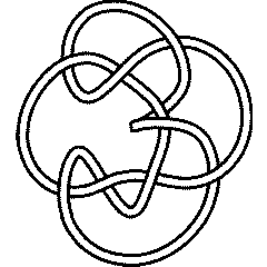
Visit 9 21's page at the Knot Server (KnotPlot driven, includes 3D interactive images!) Visit 9 21's page at Knotilus! Visit 9 21's page at the original Knot Atlas! 9 21 Quick Notes

9 21 Further Notes and Views

Knot presentations

Planar diagram presentation	X1425 X9,12,10,13 X3,11,4,10 X11,3,12,2 X13,1,14,18 X5,15,6,14 X17,7,18,6 X7,17,8,16 X15,9,16,8
Gauss code	-1, 4, -3, 1, -6, 7, -8, 9, -2, 3, -4, 2, -5, 6, -9, 8, -7, 5
Dowker-Thistlethwaite code	4 10 14 16 12 2 18 8 6
Conway Notation	[31122]

Three dimensional invariants

Symmetry type Reversible Unknotting number 1 3-genus 2 Bridge index 2 Super bridge index [math]\displaystyle{ \{4,7\} }[/math] Nakanishi index 1 Maximal Thurston-Bennequin number [-1][-10] Hyperbolic Volume 10.1833 A-Polynomial See Data:9 21/A-polynomial

[edit Notes for 9 21's three dimensional invariants]

Four dimensional invariants

Smooth 4 genus [math]\displaystyle{ 1 }[/math] Topological 4 genus [math]\displaystyle{ 1 }[/math] Concordance genus [math]\displaystyle{ 2 }[/math] Rasmussen s-Invariant 2

[edit Notes for 9 21's four dimensional invariants]

Polynomial invariants

Alexander polynomial	[math]\displaystyle{ -2 t^2+11 t-17+11 t^{-1} -2 t^{-2} }[/math]
Conway polynomial	[math]\displaystyle{ -2 z^4+3 z^2+1 }[/math]
2nd Alexander ideal (db, data sources)	[math]\displaystyle{ \{1\} }[/math]
Determinant and Signature	{ 43, 2 }
Jones polynomial	[math]\displaystyle{ -q^8+2 q^7-4 q^6+6 q^5-7 q^4+8 q^3-6 q^2+5 q-3+ q^{-1} }[/math]
HOMFLY-PT polynomial (db, data sources)	[math]\displaystyle{ -z^4 a^{-2} -z^4 a^{-4} +2 z^2 a^{-6} +z^2+ a^{-2} + a^{-6} - a^{-8} }[/math]
Kauffman polynomial (db, data sources)	[math]\displaystyle{ z^8 a^{-4} +z^8 a^{-6} +3 z^7 a^{-3} +5 z^7 a^{-5} +2 z^7 a^{-7} +4 z^6 a^{-2} +4 z^6 a^{-4} +2 z^6 a^{-6} +2 z^6 a^{-8} +3 z^5 a^{-1} -3 z^5 a^{-3} -10 z^5 a^{-5} -3 z^5 a^{-7} +z^5 a^{-9} -6 z^4 a^{-2} -9 z^4 a^{-4} -7 z^4 a^{-6} -5 z^4 a^{-8} +z^4-4 z^3 a^{-1} +2 z^3 a^{-3} +9 z^3 a^{-5} -3 z^3 a^{-9} +3 z^2 a^{-2} +6 z^2 a^{-4} +5 z^2 a^{-6} +3 z^2 a^{-8} -z^2-z a^{-3} -3 z a^{-5} +2 z a^{-9} - a^{-2} - a^{-6} - a^{-8} }[/math]
The A2 invariant	[math]\displaystyle{ q^4-q^2-1+2 q^{-2} - q^{-4} +2 q^{-6} + q^{-8} + q^{-12} - q^{-14} +2 q^{-16} - q^{-20} + q^{-22} - q^{-24} - q^{-26} }[/math]
The G2 invariant	[math]\displaystyle{ q^{18}-2 q^{16}+4 q^{14}-6 q^{12}+4 q^{10}-q^8-4 q^6+13 q^4-17 q^2+22-19 q^{-2} +5 q^{-4} +10 q^{-6} -27 q^{-8} +38 q^{-10} -39 q^{-12} +28 q^{-14} -7 q^{-16} -17 q^{-18} +36 q^{-20} -40 q^{-22} +30 q^{-24} -9 q^{-26} -13 q^{-28} +24 q^{-30} -21 q^{-32} +8 q^{-34} +18 q^{-36} -33 q^{-38} +40 q^{-40} -24 q^{-42} -4 q^{-44} +36 q^{-46} -58 q^{-48} +63 q^{-50} -46 q^{-52} +17 q^{-54} +18 q^{-56} -45 q^{-58} +57 q^{-60} -50 q^{-62} +27 q^{-64} -25 q^{-68} +32 q^{-70} -23 q^{-72} +7 q^{-74} +16 q^{-76} -28 q^{-78} +26 q^{-80} -10 q^{-82} -14 q^{-84} +36 q^{-86} -44 q^{-88} +36 q^{-90} -17 q^{-92} -8 q^{-94} +27 q^{-96} -37 q^{-98} +35 q^{-100} -23 q^{-102} +6 q^{-104} +6 q^{-106} -16 q^{-108} +16 q^{-110} -14 q^{-112} +9 q^{-114} -3 q^{-116} -2 q^{-118} +3 q^{-120} -4 q^{-122} +3 q^{-124} - q^{-126} + q^{-128} }[/math]

Further Quantum Invariants

Further quantum knot invariants for 9_21.

A1 Invariants.

Weight	Invariant
1	[math]\displaystyle{ q^3-2 q+2 q^{-1} - q^{-3} +2 q^{-5} + q^{-7} - q^{-9} +2 q^{-11} -2 q^{-13} + q^{-15} - q^{-17} }[/math]
2	[math]\displaystyle{ q^{10}-2 q^8-q^6+6 q^4-4 q^2-5+11 q^{-2} -3 q^{-4} -9 q^{-6} +11 q^{-8} + q^{-10} -8 q^{-12} +5 q^{-14} +4 q^{-16} -2 q^{-18} -5 q^{-20} +6 q^{-22} +5 q^{-24} -11 q^{-26} +3 q^{-28} +8 q^{-30} -11 q^{-32} - q^{-34} +8 q^{-36} -5 q^{-38} -2 q^{-40} +4 q^{-42} - q^{-44} - q^{-46} + q^{-48} }[/math]
3	[math]\displaystyle{ q^{21}-2 q^{19}-q^{17}+3 q^{15}+3 q^{13}-4 q^{11}-8 q^9+8 q^7+13 q^5-9 q^3-21 q+7 q^{-1} +32 q^{-3} -3 q^{-5} -40 q^{-7} -5 q^{-9} +46 q^{-11} +14 q^{-13} -41 q^{-15} -22 q^{-17} +38 q^{-19} +26 q^{-21} -25 q^{-23} -28 q^{-25} +13 q^{-27} +25 q^{-29} +2 q^{-31} -21 q^{-33} -16 q^{-35} +20 q^{-37} +26 q^{-39} -12 q^{-41} -38 q^{-43} +6 q^{-45} +42 q^{-47} + q^{-49} -46 q^{-51} -10 q^{-53} +41 q^{-55} +19 q^{-57} -36 q^{-59} -24 q^{-61} +24 q^{-63} +27 q^{-65} -13 q^{-67} -23 q^{-69} +5 q^{-71} +17 q^{-73} + q^{-75} -11 q^{-77} -2 q^{-79} +6 q^{-81} +2 q^{-83} -3 q^{-85} - q^{-87} + q^{-89} + q^{-91} - q^{-93} }[/math]
4	[math]\displaystyle{ q^{36}-2 q^{34}-q^{32}+3 q^{30}+3 q^{26}-7 q^{24}-3 q^{22}+9 q^{20}+q^{18}+9 q^{16}-22 q^{14}-16 q^{12}+22 q^{10}+21 q^8+29 q^6-50 q^4-59 q^2+16+62 q^{-2} +97 q^{-4} -54 q^{-6} -135 q^{-8} -51 q^{-10} +79 q^{-12} +191 q^{-14} +6 q^{-16} -168 q^{-18} -144 q^{-20} +28 q^{-22} +231 q^{-24} +92 q^{-26} -118 q^{-28} -179 q^{-30} -51 q^{-32} +173 q^{-34} +128 q^{-36} -27 q^{-38} -136 q^{-40} -97 q^{-42} +68 q^{-44} +109 q^{-46} +52 q^{-48} -59 q^{-50} -104 q^{-52} -38 q^{-54} +77 q^{-56} +114 q^{-58} +5 q^{-60} -107 q^{-62} -126 q^{-64} +47 q^{-66} +162 q^{-68} +69 q^{-70} -94 q^{-72} -198 q^{-74} -2 q^{-76} +178 q^{-78} +135 q^{-80} -42 q^{-82} -224 q^{-84} -75 q^{-86} +123 q^{-88} +168 q^{-90} +50 q^{-92} -170 q^{-94} -123 q^{-96} +20 q^{-98} +125 q^{-100} +110 q^{-102} -65 q^{-104} -96 q^{-106} -50 q^{-108} +42 q^{-110} +91 q^{-112} +4 q^{-114} -33 q^{-116} -47 q^{-118} -8 q^{-120} +39 q^{-122} +13 q^{-124} + q^{-126} -19 q^{-128} -11 q^{-130} +11 q^{-132} +3 q^{-134} +4 q^{-136} -4 q^{-138} -4 q^{-140} +3 q^{-142} + q^{-146} - q^{-148} - q^{-150} + q^{-152} }[/math]
5	[math]\displaystyle{ q^{55}-2 q^{53}-q^{51}+3 q^{49}-2 q^{41}-2 q^{39}+5 q^{37}+4 q^{35}-6 q^{33}-8 q^{31}-5 q^{29}+6 q^{27}+18 q^{25}+24 q^{23}-3 q^{21}-46 q^{19}-51 q^{17}-10 q^{15}+62 q^{13}+109 q^{11}+65 q^9-75 q^7-195 q^5-154 q^3+44 q+271 q^{-1} +307 q^{-3} +54 q^{-5} -326 q^{-7} -489 q^{-9} -214 q^{-11} +313 q^{-13} +652 q^{-15} +448 q^{-17} -214 q^{-19} -771 q^{-21} -680 q^{-23} +38 q^{-25} +782 q^{-27} +884 q^{-29} +188 q^{-31} -703 q^{-33} -984 q^{-35} -407 q^{-37} +529 q^{-39} +991 q^{-41} +568 q^{-43} -320 q^{-45} -875 q^{-47} -655 q^{-49} +101 q^{-51} +710 q^{-53} +657 q^{-55} +70 q^{-57} -492 q^{-59} -598 q^{-61} -214 q^{-63} +299 q^{-65} +509 q^{-67} +303 q^{-69} -122 q^{-71} -417 q^{-73} -373 q^{-75} -36 q^{-77} +353 q^{-79} +446 q^{-81} +147 q^{-83} -302 q^{-85} -520 q^{-87} -281 q^{-89} +266 q^{-91} +622 q^{-93} +398 q^{-95} -228 q^{-97} -701 q^{-99} -552 q^{-101} +156 q^{-103} +774 q^{-105} +703 q^{-107} -39 q^{-109} -782 q^{-111} -844 q^{-113} -126 q^{-115} +722 q^{-117} +932 q^{-119} +326 q^{-121} -568 q^{-123} -957 q^{-125} -506 q^{-127} +348 q^{-129} +865 q^{-131} +645 q^{-133} -88 q^{-135} -699 q^{-137} -689 q^{-139} -133 q^{-141} +458 q^{-143} +632 q^{-145} +303 q^{-147} -218 q^{-149} -501 q^{-151} -364 q^{-153} +17 q^{-155} +324 q^{-157} +340 q^{-159} +111 q^{-161} -160 q^{-163} -263 q^{-165} -154 q^{-167} +40 q^{-169} +161 q^{-171} +142 q^{-173} +28 q^{-175} -80 q^{-177} -102 q^{-179} -46 q^{-181} +26 q^{-183} +60 q^{-185} +38 q^{-187} - q^{-189} -27 q^{-191} -27 q^{-193} -5 q^{-195} +13 q^{-197} +12 q^{-199} +3 q^{-201} - q^{-203} -6 q^{-205} -4 q^{-207} +3 q^{-209} +2 q^{-211} - q^{-213} - q^{-219} + q^{-221} + q^{-223} - q^{-225} }[/math]

A2 Invariants.

Weight	Invariant
1,0	[math]\displaystyle{ q^4-q^2-1+2 q^{-2} - q^{-4} +2 q^{-6} + q^{-8} + q^{-12} - q^{-14} +2 q^{-16} - q^{-20} + q^{-22} - q^{-24} - q^{-26} }[/math]
1,1	[math]\displaystyle{ q^{12}-4 q^{10}+10 q^8-20 q^6+34 q^4-52 q^2+78-104 q^{-2} +124 q^{-4} -142 q^{-6} +152 q^{-8} -140 q^{-10} +113 q^{-12} -60 q^{-14} +2 q^{-16} +74 q^{-18} -150 q^{-20} +220 q^{-22} -268 q^{-24} +298 q^{-26} -297 q^{-28} +272 q^{-30} -228 q^{-32} +162 q^{-34} -89 q^{-36} +14 q^{-38} +50 q^{-40} -100 q^{-42} +136 q^{-44} -152 q^{-46} +144 q^{-48} -130 q^{-50} +106 q^{-52} -82 q^{-54} +56 q^{-56} -36 q^{-58} +23 q^{-60} -12 q^{-62} +6 q^{-64} -2 q^{-66} + q^{-68} }[/math]
2,0	[math]\displaystyle{ q^{12}-q^{10}-2 q^8+q^6+4 q^4+q^2-7- q^{-2} +8 q^{-4} -7 q^{-8} +2 q^{-10} +8 q^{-12} -4 q^{-16} +2 q^{-18} +4 q^{-20} -3 q^{-22} + q^{-24} +2 q^{-26} -2 q^{-28} +2 q^{-30} +7 q^{-32} - q^{-34} -6 q^{-36} + q^{-38} +5 q^{-40} -4 q^{-42} -9 q^{-44} + q^{-46} +5 q^{-48} - q^{-50} -4 q^{-52} +3 q^{-56} -2 q^{-60} + q^{-64} + q^{-66} }[/math]

A3 Invariants.

Weight	Invariant
0,1,0	[math]\displaystyle{ q^8-2 q^6+4 q^2-5+ q^{-2} +8 q^{-4} -8 q^{-6} - q^{-8} +9 q^{-10} -6 q^{-12} -2 q^{-14} +8 q^{-16} +2 q^{-22} +5 q^{-24} - q^{-26} -6 q^{-28} +6 q^{-30} + q^{-32} -10 q^{-34} +6 q^{-36} +2 q^{-38} -9 q^{-40} +3 q^{-42} + q^{-44} -4 q^{-46} +2 q^{-48} + q^{-50} - q^{-52} + q^{-54} }[/math]
1,0,0	[math]\displaystyle{ q^5-q^3- q^{-1} +2 q^{-3} - q^{-5} +2 q^{-7} + q^{-9} + q^{-11} + q^{-17} - q^{-19} +2 q^{-21} + q^{-25} - q^{-27} + q^{-29} - q^{-31} - q^{-33} - q^{-35} }[/math]

B2 Invariants.

Weight	Invariant
0,1	[math]\displaystyle{ q^8-2 q^6+4 q^4-6 q^2+7-9 q^{-2} +10 q^{-4} -8 q^{-6} +7 q^{-8} -3 q^{-10} +6 q^{-14} -10 q^{-16} +14 q^{-18} -16 q^{-20} +18 q^{-22} -17 q^{-24} +15 q^{-26} -10 q^{-28} +6 q^{-30} - q^{-32} -2 q^{-34} +6 q^{-36} -8 q^{-38} +9 q^{-40} -9 q^{-42} +7 q^{-44} -6 q^{-46} +4 q^{-48} -3 q^{-50} + q^{-52} - q^{-54} }[/math]
1,0	[math]\displaystyle{ q^{14}-2 q^{10}-2 q^8+2 q^6+5 q^4-6-4 q^{-2} +6 q^{-4} +9 q^{-6} -2 q^{-8} -10 q^{-10} -4 q^{-12} +8 q^{-14} +7 q^{-16} -4 q^{-18} -8 q^{-20} +2 q^{-22} +8 q^{-24} +2 q^{-26} -6 q^{-28} - q^{-30} +7 q^{-32} +5 q^{-34} -4 q^{-36} -4 q^{-38} +4 q^{-40} +6 q^{-42} -3 q^{-44} -7 q^{-46} + q^{-48} +8 q^{-50} + q^{-52} -9 q^{-54} -7 q^{-56} +6 q^{-58} +9 q^{-60} -2 q^{-62} -10 q^{-64} -4 q^{-66} +6 q^{-68} +5 q^{-70} -2 q^{-72} -5 q^{-74} - q^{-76} +3 q^{-78} +2 q^{-80} - q^{-82} - q^{-84} + q^{-88} }[/math]

G2 Invariants.

Weight

Invariant

1,0

[math]\displaystyle{ q^{18}-2 q^{16}+4 q^{14}-6 q^{12}+4 q^{10}-q^8-4 q^6+13 q^4-17 q^2+22-19 q^{-2} +5 q^{-4} +10 q^{-6} -27 q^{-8} +38 q^{-10} -39 q^{-12} +28 q^{-14} -7 q^{-16} -17 q^{-18} +36 q^{-20} -40 q^{-22} +30 q^{-24} -9 q^{-26} -13 q^{-28} +24 q^{-30} -21 q^{-32} +8 q^{-34} +18 q^{-36} -33 q^{-38} +40 q^{-40} -24 q^{-42} -4 q^{-44} +36 q^{-46} -58 q^{-48} +63 q^{-50} -46 q^{-52} +17 q^{-54} +18 q^{-56} -45 q^{-58} +57 q^{-60} -50 q^{-62} +27 q^{-64} -25 q^{-68} +32 q^{-70} -23 q^{-72} +7 q^{-74} +16 q^{-76} -28 q^{-78} +26 q^{-80} -10 q^{-82} -14 q^{-84} +36 q^{-86} -44 q^{-88} +36 q^{-90} -17 q^{-92} -8 q^{-94} +27 q^{-96} -37 q^{-98} +35 q^{-100} -23 q^{-102} +6 q^{-104} +6 q^{-106} -16 q^{-108} +16 q^{-110} -14 q^{-112} +9 q^{-114} -3 q^{-116} -2 q^{-118} +3 q^{-120} -4 q^{-122} +3 q^{-124} - q^{-126} + q^{-128} }[/math]

.

Computer Talk

The above data is available with the Mathematica package KnotTheory`, as shown in the (simulated) Mathematica session below. Your input (in red) is realistic; all else should have the same content as in a real mathematica session, but with different formatting. This Mathematica session is also available (albeit only for the knot 5_2) as the notebook PolynomialInvariantsSession.nb.

(The path below may be different on your system, and possibly also the KnotTheory` date)

In[1]:=

AppendTo[$Path, "C:/drorbn/projects/KAtlas/"]; << KnotTheory`

Loading KnotTheory` version of August 31, 2006, 11:25:27.5625. Read more at http://katlas.math.toronto.edu/wiki/KnotTheory.

In[3]:=

K = Knot["9 21"];

In[4]:=

Alexander[K][t]

KnotTheory::loading: Loading precomputed data in PD4Knots`.

Out[4]=

[math]\displaystyle{ -2 t^2+11 t-17+11 t^{-1} -2 t^{-2} }[/math]

In[5]:=

Conway[K][z]

Out[5]=

[math]\displaystyle{ -2 z^4+3 z^2+1 }[/math]

In[6]:=

Alexander[K, 2][t]

KnotTheory::credits: The program Alexander[K, r] to compute Alexander ideals was written by Jana Archibald at the University of Toronto in the summer of 2005.

Out[6]=

[math]\displaystyle{ \{1\} }[/math]

In[7]:=

{KnotDet[K], KnotSignature[K]}

Out[7]=

{ 43, 2 }

In[8]:=

Jones[K][q]

KnotTheory::loading: Loading precomputed data in Jones4Knots`.

Out[8]=

[math]\displaystyle{ -q^8+2 q^7-4 q^6+6 q^5-7 q^4+8 q^3-6 q^2+5 q-3+ q^{-1} }[/math]

In[9]:=

HOMFLYPT[K][a, z]

KnotTheory::credits: The HOMFLYPT program was written by Scott Morrison.

Out[9]=

[math]\displaystyle{ -z^4 a^{-2} -z^4 a^{-4} +2 z^2 a^{-6} +z^2+ a^{-2} + a^{-6} - a^{-8} }[/math]

In[10]:=

Kauffman[K][a, z]

KnotTheory::loading: Loading precomputed data in Kauffman4Knots`.

Out[10]=

[math]\displaystyle{ z^8 a^{-4} +z^8 a^{-6} +3 z^7 a^{-3} +5 z^7 a^{-5} +2 z^7 a^{-7} +4 z^6 a^{-2} +4 z^6 a^{-4} +2 z^6 a^{-6} +2 z^6 a^{-8} +3 z^5 a^{-1} -3 z^5 a^{-3} -10 z^5 a^{-5} -3 z^5 a^{-7} +z^5 a^{-9} -6 z^4 a^{-2} -9 z^4 a^{-4} -7 z^4 a^{-6} -5 z^4 a^{-8} +z^4-4 z^3 a^{-1} +2 z^3 a^{-3} +9 z^3 a^{-5} -3 z^3 a^{-9} +3 z^2 a^{-2} +6 z^2 a^{-4} +5 z^2 a^{-6} +3 z^2 a^{-8} -z^2-z a^{-3} -3 z a^{-5} +2 z a^{-9} - a^{-2} - a^{-6} - a^{-8} }[/math]

Vassiliev invariants

V2 and V3:

(3, 6)

V2,1 through V6,9:

V2,1 V3,1 V4,1 V4,2 V4,3 V5,1 V5,2 V5,3 V5,4 V6,1 V6,2 V6,3 V6,4 V6,5 V6,6 V6,7 V6,8 V6,9 [math]\displaystyle{ 12 }[/math] [math]\displaystyle{ 48 }[/math] [math]\displaystyle{ 72 }[/math] [math]\displaystyle{ 238 }[/math] [math]\displaystyle{ 50 }[/math] [math]\displaystyle{ 576 }[/math] [math]\displaystyle{ 1248 }[/math] [math]\displaystyle{ 192 }[/math] [math]\displaystyle{ 272 }[/math] [math]\displaystyle{ 288 }[/math] [math]\displaystyle{ 1152 }[/math] [math]\displaystyle{ 2856 }[/math] [math]\displaystyle{ 600 }[/math] [math]\displaystyle{ \frac{65311}{10} }[/math] [math]\displaystyle{ -\frac{3182}{5} }[/math] [math]\displaystyle{ \frac{18154}{5} }[/math] [math]\displaystyle{ \frac{235}{2} }[/math] [math]\displaystyle{ \frac{5631}{10} }[/math]

V_2,1 through V_6,9 were provided by Petr Dunin-Barkowski <barkovs@itep.ru>, Andrey Smirnov <asmirnov@itep.ru>, and Alexei Sleptsov <sleptsov@itep.ru> and uploaded on October 2010 by User:Drorbn. Note that they are normalized differently than V₂ and V₃.

Khovanov Homology

The coefficients of the monomials [math]\displaystyle{ t^rq^j }[/math] are shown, along with their alternating sums [math]\displaystyle{ \chi }[/math] (fixed [math]\displaystyle{ j }[/math], alternation over [math]\displaystyle{ r }[/math]). The squares with yellow highlighting are those on the "critical diagonals", where [math]\displaystyle{ j-2r=s+1 }[/math] or [math]\displaystyle{ j-2r=s-1 }[/math], where [math]\displaystyle{ s= }[/math]2 is the signature of 9 21. Nonzero entries off the critical diagonals (if any exist) are highlighted in red.

\   r    \    j   \ -2 -1 0 1 2 3 4 5 6 7 χ 17                   1 -1 15                 1   1 13               3 1   -2 11             3 1     2 9           4 3       -1 7         4 3         1 5       2 4           2 3     3 4             -1 1   1 3               2 -1   2                 -2 -3 1                   1

Integral Khovanov Homology (db, data source)

[math]\displaystyle{ \dim{\mathcal G}_{2r+i}\operatorname{KH}^r_{\mathbb Z} }[/math] [math]\displaystyle{ i=1 }[/math] [math]\displaystyle{ i=3 }[/math] [math]\displaystyle{ r=-2 }[/math] [math]\displaystyle{ {\mathbb Z} }[/math] [math]\displaystyle{ r=-1 }[/math] [math]\displaystyle{ {\mathbb Z}^{2}\oplus{\mathbb Z}_2 }[/math] [math]\displaystyle{ {\mathbb Z} }[/math] [math]\displaystyle{ r=0 }[/math] [math]\displaystyle{ {\mathbb Z}^{3}\oplus{\mathbb Z}_2^{2} }[/math] [math]\displaystyle{ {\mathbb Z}^{3} }[/math] [math]\displaystyle{ r=1 }[/math] [math]\displaystyle{ {\mathbb Z}^{4}\oplus{\mathbb Z}_2^{2} }[/math] [math]\displaystyle{ {\mathbb Z}^{2} }[/math] [math]\displaystyle{ r=2 }[/math] [math]\displaystyle{ {\mathbb Z}^{4}\oplus{\mathbb Z}_2^{4} }[/math] [math]\displaystyle{ {\mathbb Z}^{4} }[/math] [math]\displaystyle{ r=3 }[/math] [math]\displaystyle{ {\mathbb Z}^{3}\oplus{\mathbb Z}_2^{4} }[/math] [math]\displaystyle{ {\mathbb Z}^{4} }[/math] [math]\displaystyle{ r=4 }[/math] [math]\displaystyle{ {\mathbb Z}^{3}\oplus{\mathbb Z}_2^{3} }[/math] [math]\displaystyle{ {\mathbb Z}^{3} }[/math] [math]\displaystyle{ r=5 }[/math] [math]\displaystyle{ {\mathbb Z}\oplus{\mathbb Z}_2^{3} }[/math] [math]\displaystyle{ {\mathbb Z}^{3} }[/math] [math]\displaystyle{ r=6 }[/math] [math]\displaystyle{ {\mathbb Z}\oplus{\mathbb Z}_2 }[/math] [math]\displaystyle{ {\mathbb Z} }[/math] [math]\displaystyle{ r=7 }[/math] [math]\displaystyle{ {\mathbb Z}_2 }[/math] [math]\displaystyle{ {\mathbb Z} }[/math]

Computer Talk

Much of the above data can be recomputed by Mathematica using the package KnotTheory`. See A Sample KnotTheory` Session.

[math]\displaystyle{ \textrm{Include}(\textrm{ColouredJonesM.mhtml}) }[/math]

In[1]:=	<< KnotTheory`
Loading KnotTheory` (version of August 17, 2005, 14:44:34)...
In[2]:=	Crossings[Knot[9, 21]]
Out[2]=	9
In[3]:=	PD[Knot[9, 21]]
Out[3]=	PD[X[1, 4, 2, 5], X[9, 12, 10, 13], X[3, 11, 4, 10], X[11, 3, 12, 2], X[13, 1, 14, 18], X[5, 15, 6, 14], X[17, 7, 18, 6], X[7, 17, 8, 16], X[15, 9, 16, 8]]
In[4]:=	GaussCode[Knot[9, 21]]
Out[4]=	GaussCode[-1, 4, -3, 1, -6, 7, -8, 9, -2, 3, -4, 2, -5, 6, -9, 8, -7, 5]
In[5]:=	BR[Knot[9, 21]]
Out[5]=	BR[5, {1, 1, 2, -1, 2, -3, 2, 4, -3, 4}]
In[6]:=	alex = Alexander[Knot[9, 21]][t]
Out[6]=	2 11 2 -17 - -- + -- + 11 t - 2 t 2 t t
In[7]:=	Conway[Knot[9, 21]][z]
Out[7]=	2 4 1 + 3 z - 2 z
In[8]:=	Select[AllKnots[], (alex === Alexander[#][t])&]
Out[8]=	{Knot[9, 21]}
In[9]:=	{KnotDet[Knot[9, 21]], KnotSignature[Knot[9, 21]]}
Out[9]=	{43, 2}
In[10]:=	J=Jones[Knot[9, 21]][q]
Out[10]=	1 2 3 4 5 6 7 8 -3 + - + 5 q - 6 q + 8 q - 7 q + 6 q - 4 q + 2 q - q q
In[11]:=	Select[AllKnots[], (J === Jones[#][q] || (J /. q-> 1/q) === Jones[#][q])&]
Out[11]=	{Knot[9, 21], Knot[11, NonAlternating, 129]}
In[12]:=	A2Invariant[Knot[9, 21]][q]
Out[12]=	-4 -2 2 4 6 8 12 14 16 20 -1 + q - q + 2 q - q + 2 q + q + q - q + 2 q - q + 22 24 26 q - q - q
In[13]:=	Kauffman[Knot[9, 21]][a, z]
Out[13]=	2 2 2 2 -8 -6 -2 2 z 3 z z 2 3 z 5 z 6 z 3 z -a - a - a + --- - --- - -- - z + ---- + ---- + ---- + ---- - 9 5 3 8 6 4 2 a a a a a a a 3 3 3 3 4 4 4 4 5 3 z 9 z 2 z 4 z 4 5 z 7 z 9 z 6 z z ---- + ---- + ---- - ---- + z - ---- - ---- - ---- - ---- + -- - 9 5 3 a 8 6 4 2 9 a a a a a a a a 5 5 5 5 6 6 6 6 7 3 z 10 z 3 z 3 z 2 z 2 z 4 z 4 z 2 z ---- - ----- - ---- + ---- + ---- + ---- + ---- + ---- + ---- + 7 5 3 a 8 6 4 2 7 a a a a a a a a 7 7 8 8 5 z 3 z z z ---- + ---- + -- + -- 5 3 6 4 a a a a
In[14]:=	{Vassiliev[2][Knot[9, 21]], Vassiliev[3][Knot[9, 21]]}
Out[14]=	{0, 6}
In[15]:=	Kh[Knot[9, 21]][q, t]
Out[15]=	3 1 2 q 3 5 5 2 7 2 3 q + 3 q + ----- + --- + - + 4 q t + 2 q t + 4 q t + 4 q t + 3 2 q t t q t 7 3 9 3 9 4 11 4 11 5 13 5 13 6 3 q t + 4 q t + 3 q t + 3 q t + q t + 3 q t + q t + 15 6 17 7 q t + q t