10 110

10_109

10_111

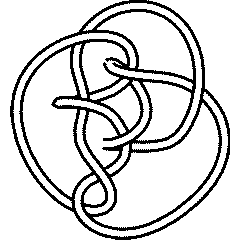
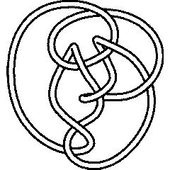
Visit 10 110's page at the Knot Server (KnotPlot driven, includes 3D interactive images!) Visit 10 110's page at Knotilus! Visit 10 110's page at the original Knot Atlas! 10 110 Quick Notes

10 110 Further Notes and Views

Knot presentations

Planar diagram presentation	X1627 X7,20,8,1 X3,11,4,10 X5,16,6,17 X17,8,18,9 X9,14,10,15 X11,3,12,2 X15,4,16,5 X13,19,14,18 X19,13,20,12
Gauss code	-1, 7, -3, 8, -4, 1, -2, 5, -6, 3, -7, 10, -9, 6, -8, 4, -5, 9, -10, 2
Dowker-Thistlethwaite code	6 10 16 20 14 2 18 4 8 12
Conway Notation	[2.2.2.20]

Three dimensional invariants

Symmetry type Chiral Unknotting number 2 3-genus 3 Bridge index 3 Super bridge index Missing Nakanishi index 1 Maximal Thurston-Bennequin number [-9][-3] Hyperbolic Volume 14.7775 A-Polynomial See Data:10 110/A-polynomial

[edit Notes for 10 110's three dimensional invariants]

Four dimensional invariants

Smooth 4 genus Failed to parse (SVG (MathML can be enabled via browser plugin): Invalid response ("Math extension cannot connect to Restbase.") from server "https://wikimedia.org/api/rest_v1/":): {\displaystyle 1} Topological 4 genus $1$ Concordance genus $3$ Rasmussen s-Invariant -2

[edit Notes for 10 110's four dimensional invariants]

Polynomial invariants

Alexander polynomial	$t^{3}-8t^{2}+20t-25+20t^{-1}-8t^{-2}+t^{-3}$
Conway polynomial	$z^{6}-2z^{4}-3z^{2}+1$
2nd Alexander ideal (db, data sources)	$\{1\}$
Determinant and Signature	{ 83, -2 }
Jones polynomial	$q^{3}-3q^{2}+7q-10+13q^{-1}-14q^{-2}+13q^{-3}-11q^{-4}+7q^{-5}-3q^{-6}+q^{-7}$
HOMFLY-PT polynomial (db, data sources)	$z^{2}a^{6}+a^{6}-2z^{4}a^{4}-3z^{2}a^{4}-a^{4}+z^{6}a^{2}+2z^{4}a^{2}+z^{2}a^{2}-2z^{4}-3z^{2}+z^{2}a^{-2}+a^{-2}$
Kauffman polynomial (db, data sources)	$2a^{3}z^{9}+2az^{9}+6a^{4}z^{8}+10a^{2}z^{8}+4z^{8}+8a^{5}z^{7}+9a^{3}z^{7}+4az^{7}+3z^{7}a^{-1}+6a^{6}z^{6}-5a^{4}z^{6}-20a^{2}z^{6}+z^{6}a^{-2}-8z^{6}+3a^{7}z^{5}-13a^{5}z^{5}-27a^{3}z^{5}-19az^{5}-8z^{5}a^{-1}+a^{8}z^{4}-7a^{6}z^{4}-4a^{4}z^{4}+8a^{2}z^{4}-3z^{4}a^{-2}+z^{4}-2a^{7}z^{3}+12a^{5}z^{3}+21a^{3}z^{3}+13az^{3}+6z^{3}a^{-1}-a^{8}z^{2}+5a^{6}z^{2}+6a^{4}z^{2}-a^{2}z^{2}+3z^{2}a^{-2}+2z^{2}-4a^{5}z-6a^{3}z-3az-za^{-1}-a^{6}-a^{4}-a^{-2}$
The A2 invariant	$q^{22}-q^{18}+3q^{16}-2q^{14}+q^{10}-3q^{8}+2q^{6}-3q^{4}+2q^{2}+1-q^{-2}+3q^{-4}-q^{-6}+q^{-10}$
The G2 invariant	$q^{114}-2q^{112}+4q^{110}-6q^{108}+6q^{106}-5q^{104}+10q^{100}-20q^{98}+31q^{96}-39q^{94}+35q^{92}-20q^{90}-10q^{88}+55q^{86}-94q^{84}+121q^{82}-118q^{80}+71q^{78}+10q^{76}-112q^{74}+200q^{72}-226q^{70}+178q^{68}-61q^{66}-84q^{64}+200q^{62}-231q^{60}+167q^{58}-31q^{56}-116q^{54}+198q^{52}-176q^{50}+53q^{48}+118q^{46}-250q^{44}+281q^{42}-194q^{40}+14q^{38}+182q^{36}-325q^{34}+358q^{32}-275q^{30}+101q^{28}+99q^{26}-256q^{24}+317q^{22}-265q^{20}+124q^{18}+44q^{16}-179q^{14}+221q^{12}-157q^{10}+20q^{8}+134q^{6}-223q^{4}+206q^{2}-87-82q^{-2}+226q^{-4}-279q^{-6}+228q^{-8}-96q^{-10}-60q^{-12}+176q^{-14}-213q^{-16}+180q^{-18}-94q^{-20}+3q^{-22}+60q^{-24}-87q^{-26}+76q^{-28}-46q^{-30}+19q^{-32}+3q^{-34}-12q^{-36}+13q^{-38}-10q^{-40}+6q^{-42}-2q^{-44}+q^{-46}$

Further Quantum Invariants

Further quantum knot invariants for 10_110.

A1 Invariants.

Weight	Invariant
1	$q^{15}-2q^{13}+4q^{11}-4q^{9}+2q^{7}-q^{5}-q^{3}+3q-3q^{-1}+4q^{-3}-2q^{-5}+q^{-7}$
2	$q^{42}-2q^{40}+q^{38}+5q^{36}-11q^{34}+3q^{32}+19q^{30}-26q^{28}-5q^{26}+37q^{24}-23q^{22}-19q^{20}+32q^{18}-2q^{16}-22q^{14}+8q^{12}+19q^{10}-13q^{8}-18q^{6}+28q^{4}+3q^{2}-35+22q^{-2}+20q^{-4}-33q^{-6}+4q^{-8}+23q^{-10}-14q^{-12}-6q^{-14}+9q^{-16}-q^{-18}-2q^{-20}+q^{-22}$
3	$q^{81}-2q^{79}+q^{77}+2q^{75}-2q^{73}-5q^{71}+6q^{69}+13q^{67}-18q^{65}-30q^{63}+34q^{61}+63q^{59}-40q^{57}-122q^{55}+31q^{53}+189q^{51}+8q^{49}-235q^{47}-84q^{45}+253q^{43}+158q^{41}-218q^{39}-215q^{37}+144q^{35}+239q^{33}-52q^{31}-227q^{29}-37q^{27}+190q^{25}+109q^{23}-140q^{21}-169q^{19}+90q^{17}+211q^{15}-36q^{13}-244q^{11}-16q^{9}+257q^{7}+86q^{5}-250q^{3}-154q+213q^{-1}+210q^{-3}-142q^{-5}-241q^{-7}+54q^{-9}+233q^{-11}+27q^{-13}-182q^{-15}-81q^{-17}+110q^{-19}+99q^{-21}-48q^{-23}-77q^{-25}+3q^{-27}+46q^{-29}+12q^{-31}-20q^{-33}-9q^{-35}+6q^{-37}+4q^{-39}-q^{-41}-2q^{-43}+q^{-45}$

A2 Invariants.

Weight	Invariant
1,0	$q^{22}-q^{18}+3q^{16}-2q^{14}+q^{10}-3q^{8}+2q^{6}-3q^{4}+2q^{2}+1-q^{-2}+3q^{-4}-q^{-6}+q^{-10}$
2,0	$q^{56}-q^{52}+q^{50}+2q^{48}-q^{46}-6q^{44}+3q^{42}+10q^{40}-9q^{38}-11q^{36}+7q^{34}+15q^{32}-10q^{30}-16q^{28}+14q^{26}+10q^{24}-10q^{22}-4q^{20}+12q^{18}-2q^{16}-3q^{14}+6q^{12}-q^{10}-9q^{8}+2q^{6}+12q^{4}-12q^{2}-10+15q^{-2}+9q^{-4}-13q^{-6}-7q^{-8}+11q^{-10}+7q^{-12}-9q^{-14}-6q^{-16}+6q^{-18}+5q^{-20}-q^{-22}-2q^{-24}+q^{-28}$

A3 Invariants.

Weight	Invariant
0,1,0	$q^{48}-2q^{46}+6q^{42}-7q^{40}-4q^{38}+18q^{36}-12q^{34}-13q^{32}+27q^{30}-13q^{28}-16q^{26}+27q^{24}-6q^{22}-11q^{20}+12q^{18}+3q^{16}-5q^{14}-10q^{12}+9q^{10}+6q^{8}-23q^{6}+9q^{4}+18q^{2}-25+8q^{-2}+17q^{-4}-20q^{-6}+8q^{-8}+8q^{-10}-9q^{-12}+4q^{-14}+2q^{-16}-2q^{-18}+q^{-20}$
1,0,0	$q^{29}+q^{25}-q^{23}+3q^{21}-3q^{19}+2q^{17}-2q^{15}+q^{13}-2q^{11}-2q^{5}+2q^{3}-q+3q^{-1}-2q^{-3}+3q^{-5}-q^{-7}+q^{-9}+q^{-13}$

B2 Invariants.

Weight	Invariant
0,1	$q^{48}-2q^{46}+4q^{44}-8q^{42}+13q^{40}-18q^{38}+26q^{36}-30q^{34}+33q^{32}-31q^{30}+25q^{28}-14q^{26}-q^{24}+16q^{22}-33q^{20}+46q^{18}-59q^{16}+63q^{14}-62q^{12}+55q^{10}-42q^{8}+27q^{6}-9q^{4}-6q^{2}+19-28q^{-2}+33q^{-4}-32q^{-6}+30q^{-8}-24q^{-10}+17q^{-12}-10q^{-14}+6q^{-16}-2q^{-18}+q^{-20}$
1,0	Failed to parse (SVG (MathML can be enabled via browser plugin): Invalid response ("Math extension cannot connect to Restbase.") from server "https://wikimedia.org/api/rest_v1/":): {\displaystyle q^{78}-2 q^{74}-2 q^{72}+2 q^{70}+7 q^{68}+2 q^{66}-10 q^{64}-11 q^{62}+5 q^{60}+22 q^{58}+7 q^{56}-23 q^{54}-23 q^{52}+12 q^{50}+33 q^{48}+3 q^{46}-33 q^{44}-17 q^{42}+25 q^{40}+26 q^{38}-13 q^{36}-27 q^{34}+5 q^{32}+27 q^{30}+4 q^{28}-24 q^{26}-8 q^{24}+19 q^{22}+12 q^{20}-17 q^{18}-17 q^{16}+14 q^{14}+21 q^{12}-11 q^{10}-30 q^8+q^6+33 q^4+15 q^2-28-29 q^{-2} +16 q^{-4} +35 q^{-6} + q^{-8} -28 q^{-10} -14 q^{-12} +18 q^{-14} +18 q^{-16} -5 q^{-18} -13 q^{-20} -2 q^{-22} +7 q^{-24} +4 q^{-26} -2 q^{-28} -2 q^{-30} + q^{-34} }

G2 Invariants.

Weight

Invariant

1,0

Failed to parse (SVG (MathML can be enabled via browser plugin): Invalid response ("Math extension cannot connect to Restbase.") from server "https://wikimedia.org/api/rest_v1/":): {\displaystyle q^{114}-2 q^{112}+4 q^{110}-6 q^{108}+6 q^{106}-5 q^{104}+10 q^{100}-20 q^{98}+31 q^{96}-39 q^{94}+35 q^{92}-20 q^{90}-10 q^{88}+55 q^{86}-94 q^{84}+121 q^{82}-118 q^{80}+71 q^{78}+10 q^{76}-112 q^{74}+200 q^{72}-226 q^{70}+178 q^{68}-61 q^{66}-84 q^{64}+200 q^{62}-231 q^{60}+167 q^{58}-31 q^{56}-116 q^{54}+198 q^{52}-176 q^{50}+53 q^{48}+118 q^{46}-250 q^{44}+281 q^{42}-194 q^{40}+14 q^{38}+182 q^{36}-325 q^{34}+358 q^{32}-275 q^{30}+101 q^{28}+99 q^{26}-256 q^{24}+317 q^{22}-265 q^{20}+124 q^{18}+44 q^{16}-179 q^{14}+221 q^{12}-157 q^{10}+20 q^8+134 q^6-223 q^4+206 q^2-87-82 q^{-2} +226 q^{-4} -279 q^{-6} +228 q^{-8} -96 q^{-10} -60 q^{-12} +176 q^{-14} -213 q^{-16} +180 q^{-18} -94 q^{-20} +3 q^{-22} +60 q^{-24} -87 q^{-26} +76 q^{-28} -46 q^{-30} +19 q^{-32} +3 q^{-34} -12 q^{-36} +13 q^{-38} -10 q^{-40} +6 q^{-42} -2 q^{-44} + q^{-46} }

.

Computer Talk

The above data is available with the Mathematica package KnotTheory`, as shown in the (simulated) Mathematica session below. Your input (in red) is realistic; all else should have the same content as in a real mathematica session, but with different formatting. This Mathematica session is also available (albeit only for the knot 5_2) as the notebook PolynomialInvariantsSession.nb.

(The path below may be different on your system, and possibly also the KnotTheory` date)

In[1]:=

AppendTo[$Path, "C:/drorbn/projects/KAtlas/"]; << KnotTheory`

Loading KnotTheory` version of August 31, 2006, 11:25:27.5625. Read more at http://katlas.math.toronto.edu/wiki/KnotTheory.

In[3]:=

K = Knot["10 110"];

In[4]:=

Alexander[K][t]

KnotTheory::loading: Loading precomputed data in PD4Knots`.

Out[4]=

$t^{3}-8t^{2}+20t-25+20t^{-1}-8t^{-2}+t^{-3}$

In[5]:=

Conway[K][z]

Out[5]=

$z^{6}-2z^{4}-3z^{2}+1$

In[6]:=

Alexander[K, 2][t]

KnotTheory::credits: The program Alexander[K, r] to compute Alexander ideals was written by Jana Archibald at the University of Toronto in the summer of 2005.

Out[6]=

$\{1\}$

In[7]:=

{KnotDet[K], KnotSignature[K]}

Out[7]=

{ 83, -2 }

In[8]:=

Jones[K][q]

KnotTheory::loading: Loading precomputed data in Jones4Knots`.

Out[8]=

$q^{3}-3q^{2}+7q-10+13q^{-1}-14q^{-2}+13q^{-3}-11q^{-4}+7q^{-5}-3q^{-6}+q^{-7}$

In[9]:=

HOMFLYPT[K][a, z]

KnotTheory::credits: The HOMFLYPT program was written by Scott Morrison.

Out[9]=

$z^{2}a^{6}+a^{6}-2z^{4}a^{4}-3z^{2}a^{4}-a^{4}+z^{6}a^{2}+2z^{4}a^{2}+z^{2}a^{2}-2z^{4}-3z^{2}+z^{2}a^{-2}+a^{-2}$

In[10]:=

Kauffman[K][a, z]

KnotTheory::loading: Loading precomputed data in Kauffman4Knots`.

Out[10]=

$2a^{3}z^{9}+2az^{9}+6a^{4}z^{8}+10a^{2}z^{8}+4z^{8}+8a^{5}z^{7}+9a^{3}z^{7}+4az^{7}+3z^{7}a^{-1}+6a^{6}z^{6}-5a^{4}z^{6}-20a^{2}z^{6}+z^{6}a^{-2}-8z^{6}+3a^{7}z^{5}-13a^{5}z^{5}-27a^{3}z^{5}-19az^{5}-8z^{5}a^{-1}+a^{8}z^{4}-7a^{6}z^{4}-4a^{4}z^{4}+8a^{2}z^{4}-3z^{4}a^{-2}+z^{4}-2a^{7}z^{3}+12a^{5}z^{3}+21a^{3}z^{3}+13az^{3}+6z^{3}a^{-1}-a^{8}z^{2}+5a^{6}z^{2}+6a^{4}z^{2}-a^{2}z^{2}+3z^{2}a^{-2}+2z^{2}-4a^{5}z-6a^{3}z-3az-za^{-1}-a^{6}-a^{4}-a^{-2}$

Vassiliev invariants

V2 and V3:

(-3, 3)

V2,1 through V6,9:

V2,1 V3,1 V4,1 V4,2 V4,3 V5,1 V5,2 V5,3 V5,4 V6,1 V6,2 V6,3 V6,4 V6,5 V6,6 V6,7 V6,8 V6,9 Failed to parse (SVG (MathML can be enabled via browser plugin): Invalid response ("Math extension cannot connect to Restbase.") from server "https://wikimedia.org/api/rest_v1/":): {\displaystyle -12} Failed to parse (SVG (MathML can be enabled via browser plugin): Invalid response ("Math extension cannot connect to Restbase.") from server "https://wikimedia.org/api/rest_v1/":): {\displaystyle 24} Failed to parse (SVG (MathML can be enabled via browser plugin): Invalid response ("Math extension cannot connect to Restbase.") from server "https://wikimedia.org/api/rest_v1/":): {\displaystyle 72} Failed to parse (SVG (MathML can be enabled via browser plugin): Invalid response ("Math extension cannot connect to Restbase.") from server "https://wikimedia.org/api/rest_v1/":): {\displaystyle 82} Failed to parse (SVG (MathML can be enabled via browser plugin): Invalid response ("Math extension cannot connect to Restbase.") from server "https://wikimedia.org/api/rest_v1/":): {\displaystyle 54} Failed to parse (SVG (MathML can be enabled via browser plugin): Invalid response ("Math extension cannot connect to Restbase.") from server "https://wikimedia.org/api/rest_v1/":): {\displaystyle -288} Failed to parse (SVG (MathML can be enabled via browser plugin): Invalid response ("Math extension cannot connect to Restbase.") from server "https://wikimedia.org/api/rest_v1/":): {\displaystyle -464} $-128$ Failed to parse (SVG (MathML can be enabled via browser plugin): Invalid response ("Math extension cannot connect to Restbase.") from server "https://wikimedia.org/api/rest_v1/":): {\displaystyle -104} Failed to parse (SVG (MathML can be enabled via browser plugin): Invalid response ("Math extension cannot connect to Restbase.") from server "https://wikimedia.org/api/rest_v1/":): {\displaystyle -288} Failed to parse (SVG (MathML can be enabled via browser plugin): Invalid response ("Math extension cannot connect to Restbase.") from server "https://wikimedia.org/api/rest_v1/":): {\displaystyle 288} Failed to parse (SVG (MathML can be enabled via browser plugin): Invalid response ("Math extension cannot connect to Restbase.") from server "https://wikimedia.org/api/rest_v1/":): {\displaystyle -984} Failed to parse (SVG (MathML can be enabled via browser plugin): Invalid response ("Math extension cannot connect to Restbase.") from server "https://wikimedia.org/api/rest_v1/":): {\displaystyle -648} Failed to parse (SVG (MathML can be enabled via browser plugin): Invalid response ("Math extension cannot connect to Restbase.") from server "https://wikimedia.org/api/rest_v1/":): {\displaystyle -\frac{511}{10}} Failed to parse (SVG (MathML can be enabled via browser plugin): Invalid response ("Math extension cannot connect to Restbase.") from server "https://wikimedia.org/api/rest_v1/":): {\displaystyle \frac{5906}{15}} Failed to parse (SVG (MathML can be enabled via browser plugin): Invalid response ("Math extension cannot connect to Restbase.") from server "https://wikimedia.org/api/rest_v1/":): {\displaystyle -\frac{12742}{15}} ${\frac {1343}{6}}$ Failed to parse (SVG (MathML can be enabled via browser plugin): Invalid response ("Math extension cannot connect to Restbase.") from server "https://wikimedia.org/api/rest_v1/":): {\displaystyle -\frac{2591}{10}}

V_2,1 through V_6,9 were provided by Petr Dunin-Barkowski <barkovs@itep.ru>, Andrey Smirnov <asmirnov@itep.ru>, and Alexei Sleptsov <sleptsov@itep.ru> and uploaded on October 2010 by User:Drorbn. Note that they are normalized differently than V₂ and V₃.

Khovanov Homology

The coefficients of the monomials Failed to parse (SVG (MathML can be enabled via browser plugin): Invalid response ("Math extension cannot connect to Restbase.") from server "https://wikimedia.org/api/rest_v1/":): {\displaystyle t^rq^j} are shown, along with their alternating sums Failed to parse (SVG (MathML can be enabled via browser plugin): Invalid response ("Math extension cannot connect to Restbase.") from server "https://wikimedia.org/api/rest_v1/":): {\displaystyle \chi} (fixed Failed to parse (SVG (MathML can be enabled via browser plugin): Invalid response ("Math extension cannot connect to Restbase.") from server "https://wikimedia.org/api/rest_v1/":): {\displaystyle j} , alternation over Failed to parse (SVG (MathML can be enabled via browser plugin): Invalid response ("Math extension cannot connect to Restbase.") from server "https://wikimedia.org/api/rest_v1/":): {\displaystyle r} ). The squares with yellow highlighting are those on the "critical diagonals", where Failed to parse (SVG (MathML can be enabled via browser plugin): Invalid response ("Math extension cannot connect to Restbase.") from server "https://wikimedia.org/api/rest_v1/":): {\displaystyle j-2r=s+1} or Failed to parse (SVG (MathML can be enabled via browser plugin): Invalid response ("Math extension cannot connect to Restbase.") from server "https://wikimedia.org/api/rest_v1/":): {\displaystyle j-2r=s-1} , where Failed to parse (SVG (MathML can be enabled via browser plugin): Invalid response ("Math extension cannot connect to Restbase.") from server "https://wikimedia.org/api/rest_v1/":): {\displaystyle s=} -2 is the signature of 10 110. Nonzero entries off the critical diagonals (if any exist) are highlighted in red.

\   r    \    j   \ -6 -5 -4 -3 -2 -1 0 1 2 3 4 χ 7                     1 1 5                   2   -2 3                 5 1   4 1               5 2     -3 -1             8 5       3 -3           7 6         -1 -5         6 7           -1 -7       5 7             2 -9     2 6               -4 -11   1 5                 4 -13   2                   -2 -15 1                     1

Integral Khovanov Homology (db, data source)

$\dim {\mathcal {G}}_{2r+i}\operatorname {KH} _{\mathbb {Z} }^{r}$ Failed to parse (SVG (MathML can be enabled via browser plugin): Invalid response ("Math extension cannot connect to Restbase.") from server "https://wikimedia.org/api/rest_v1/":): {\displaystyle i=-3} Failed to parse (SVG (MathML can be enabled via browser plugin): Invalid response ("Math extension cannot connect to Restbase.") from server "https://wikimedia.org/api/rest_v1/":): {\displaystyle i=-1} Failed to parse (SVG (MathML can be enabled via browser plugin): Invalid response ("Math extension cannot connect to Restbase.") from server "https://wikimedia.org/api/rest_v1/":): {\displaystyle r=-6} Failed to parse (SVG (MathML can be enabled via browser plugin): Invalid response ("Math extension cannot connect to Restbase.") from server "https://wikimedia.org/api/rest_v1/":): {\displaystyle {\mathbb Z}} Failed to parse (SVG (MathML can be enabled via browser plugin): Invalid response ("Math extension cannot connect to Restbase.") from server "https://wikimedia.org/api/rest_v1/":): {\displaystyle r=-5} Failed to parse (SVG (MathML can be enabled via browser plugin): Invalid response ("Math extension cannot connect to Restbase.") from server "https://wikimedia.org/api/rest_v1/":): {\displaystyle {\mathbb Z}^{2}\oplus{\mathbb Z}_2} Failed to parse (SVG (MathML can be enabled via browser plugin): Invalid response ("Math extension cannot connect to Restbase.") from server "https://wikimedia.org/api/rest_v1/":): {\displaystyle {\mathbb Z}} Failed to parse (SVG (MathML can be enabled via browser plugin): Invalid response ("Math extension cannot connect to Restbase.") from server "https://wikimedia.org/api/rest_v1/":): {\displaystyle r=-4} Failed to parse (SVG (MathML can be enabled via browser plugin): Invalid response ("Math extension cannot connect to Restbase.") from server "https://wikimedia.org/api/rest_v1/":): {\displaystyle {\mathbb Z}^{5}\oplus{\mathbb Z}_2^{2}} Failed to parse (SVG (MathML can be enabled via browser plugin): Invalid response ("Math extension cannot connect to Restbase.") from server "https://wikimedia.org/api/rest_v1/":): {\displaystyle {\mathbb Z}^{2}} Failed to parse (SVG (MathML can be enabled via browser plugin): Invalid response ("Math extension cannot connect to Restbase.") from server "https://wikimedia.org/api/rest_v1/":): {\displaystyle r=-3} ${\mathbb {Z} }^{6}\oplus {\mathbb {Z} }_{2}^{5}$ Failed to parse (SVG (MathML can be enabled via browser plugin): Invalid response ("Math extension cannot connect to Restbase.") from server "https://wikimedia.org/api/rest_v1/":): {\displaystyle {\mathbb Z}^{5}} Failed to parse (SVG (MathML can be enabled via browser plugin): Invalid response ("Math extension cannot connect to Restbase.") from server "https://wikimedia.org/api/rest_v1/":): {\displaystyle r=-2} Failed to parse (SVG (MathML can be enabled via browser plugin): Invalid response ("Math extension cannot connect to Restbase.") from server "https://wikimedia.org/api/rest_v1/":): {\displaystyle {\mathbb Z}^{7}\oplus{\mathbb Z}_2^{6}} Failed to parse (SVG (MathML can be enabled via browser plugin): Invalid response ("Math extension cannot connect to Restbase.") from server "https://wikimedia.org/api/rest_v1/":): {\displaystyle {\mathbb Z}^{6}} Failed to parse (SVG (MathML can be enabled via browser plugin): Invalid response ("Math extension cannot connect to Restbase.") from server "https://wikimedia.org/api/rest_v1/":): {\displaystyle r=-1} Failed to parse (SVG (MathML can be enabled via browser plugin): Invalid response ("Math extension cannot connect to Restbase.") from server "https://wikimedia.org/api/rest_v1/":): {\displaystyle {\mathbb Z}^{7}\oplus{\mathbb Z}_2^{7}} Failed to parse (SVG (MathML can be enabled via browser plugin): Invalid response ("Math extension cannot connect to Restbase.") from server "https://wikimedia.org/api/rest_v1/":): {\displaystyle {\mathbb Z}^{7}} Failed to parse (SVG (MathML can be enabled via browser plugin): Invalid response ("Math extension cannot connect to Restbase.") from server "https://wikimedia.org/api/rest_v1/":): {\displaystyle r=0} Failed to parse (SVG (MathML can be enabled via browser plugin): Invalid response ("Math extension cannot connect to Restbase.") from server "https://wikimedia.org/api/rest_v1/":): {\displaystyle {\mathbb Z}^{6}\oplus{\mathbb Z}_2^{7}} Failed to parse (SVG (MathML can be enabled via browser plugin): Invalid response ("Math extension cannot connect to Restbase.") from server "https://wikimedia.org/api/rest_v1/":): {\displaystyle {\mathbb Z}^{8}} Failed to parse (SVG (MathML can be enabled via browser plugin): Invalid response ("Math extension cannot connect to Restbase.") from server "https://wikimedia.org/api/rest_v1/":): {\displaystyle r=1} Failed to parse (SVG (MathML can be enabled via browser plugin): Invalid response ("Math extension cannot connect to Restbase.") from server "https://wikimedia.org/api/rest_v1/":): {\displaystyle {\mathbb Z}^{5}\oplus{\mathbb Z}_2^{5}} Failed to parse (SVG (MathML can be enabled via browser plugin): Invalid response ("Math extension cannot connect to Restbase.") from server "https://wikimedia.org/api/rest_v1/":): {\displaystyle {\mathbb Z}^{5}} Failed to parse (SVG (MathML can be enabled via browser plugin): Invalid response ("Math extension cannot connect to Restbase.") from server "https://wikimedia.org/api/rest_v1/":): {\displaystyle r=2} Failed to parse (SVG (MathML can be enabled via browser plugin): Invalid response ("Math extension cannot connect to Restbase.") from server "https://wikimedia.org/api/rest_v1/":): {\displaystyle {\mathbb Z}^{2}\oplus{\mathbb Z}_2^{5}} Failed to parse (SVG (MathML can be enabled via browser plugin): Invalid response ("Math extension cannot connect to Restbase.") from server "https://wikimedia.org/api/rest_v1/":): {\displaystyle {\mathbb Z}^{5}} Failed to parse (SVG (MathML can be enabled via browser plugin): Invalid response ("Math extension cannot connect to Restbase.") from server "https://wikimedia.org/api/rest_v1/":): {\displaystyle r=3} Failed to parse (SVG (MathML can be enabled via browser plugin): Invalid response ("Math extension cannot connect to Restbase.") from server "https://wikimedia.org/api/rest_v1/":): {\displaystyle {\mathbb Z}\oplus{\mathbb Z}_2^{2}} Failed to parse (SVG (MathML can be enabled via browser plugin): Invalid response ("Math extension cannot connect to Restbase.") from server "https://wikimedia.org/api/rest_v1/":): {\displaystyle {\mathbb Z}^{2}} Failed to parse (SVG (MathML can be enabled via browser plugin): Invalid response ("Math extension cannot connect to Restbase.") from server "https://wikimedia.org/api/rest_v1/":): {\displaystyle r=4} Failed to parse (SVG (MathML can be enabled via browser plugin): Invalid response ("Math extension cannot connect to Restbase.") from server "https://wikimedia.org/api/rest_v1/":): {\displaystyle {\mathbb Z}_2} Failed to parse (SVG (MathML can be enabled via browser plugin): Invalid response ("Math extension cannot connect to Restbase.") from server "https://wikimedia.org/api/rest_v1/":): {\displaystyle {\mathbb Z}}

Computer Talk

Much of the above data can be recomputed by Mathematica using the package KnotTheory`. See A Sample KnotTheory` Session.

Failed to parse (SVG (MathML can be enabled via browser plugin): Invalid response ("Math extension cannot connect to Restbase.") from server "https://wikimedia.org/api/rest_v1/":): {\displaystyle \textrm{Include}(\textrm{ColouredJonesM.mhtml})}

In[1]:=	<< KnotTheory`
Loading KnotTheory` (version of August 17, 2005, 14:44:34)...
In[2]:=	Crossings[Knot[10, 110]]
Out[2]=	10
In[3]:=	PD[Knot[10, 110]]
Out[3]=	PD[X[1, 6, 2, 7], X[7, 20, 8, 1], X[3, 11, 4, 10], X[5, 16, 6, 17], X[17, 8, 18, 9], X[9, 14, 10, 15], X[11, 3, 12, 2], X[15, 4, 16, 5], X[13, 19, 14, 18], X[19, 13, 20, 12]]
In[4]:=	GaussCode[Knot[10, 110]]
Out[4]=	GaussCode[-1, 7, -3, 8, -4, 1, -2, 5, -6, 3, -7, 10, -9, 6, -8, 4, -5, 9, -10, 2]
In[5]:=	BR[Knot[10, 110]]
Out[5]=	BR[5, {-1, 2, -1, -3, -2, -2, -2, 4, 3, -2, 3, 4}]
In[6]:=	alex = Alexander[Knot[10, 110]][t]
Out[6]=	-3 8 20 2 3 -25 + t - -- + -- + 20 t - 8 t + t 2 t t
In[7]:=	Conway[Knot[10, 110]][z]
Out[7]=	2 4 6 1 - 3 z - 2 z + z
In[8]:=	Select[AllKnots[], (alex === Alexander[#][t])&]
Out[8]=	{Knot[10, 110]}
In[9]:=	{KnotDet[Knot[10, 110]], KnotSignature[Knot[10, 110]]}
Out[9]=	{83, -2}
In[10]:=	J=Jones[Knot[10, 110]][q]
Out[10]=	-7 3 7 11 13 14 13 2 3 -10 + q - -- + -- - -- + -- - -- + -- + 7 q - 3 q + q 6 5 4 3 2 q q q q q q
In[11]:=	Select[AllKnots[], (J === Jones[#][q] || (J /. q-> 1/q) === Jones[#][q])&]
Out[11]=	{Knot[10, 110]}
In[12]:=	A2Invariant[Knot[10, 110]][q]
Out[12]=	-22 -18 3 2 -10 3 2 3 2 2 4 1 + q - q + --- - --- + q - -- + -- - -- + -- - q + 3 q - 16 14 8 6 4 2 q q q q q q 6 10 q + q
In[13]:=	Kauffman[Knot[10, 110]][a, z]
Out[13]=	2 -2 4 6 z 3 5 2 3 z 2 2 -a - a - a - - - 3 a z - 6 a z - 4 a z + 2 z + ---- - a z + a 2 a 3 4 2 6 2 8 2 6 z 3 3 3 5 3 6 a z + 5 a z - a z + ---- + 13 a z + 21 a z + 12 a z - a 4 5 7 3 4 3 z 2 4 4 4 6 4 8 4 8 z 2 a z + z - ---- + 8 a z - 4 a z - 7 a z + a z - ---- - 2 a a 6 5 3 5 5 5 7 5 6 z 2 6 19 a z - 27 a z - 13 a z + 3 a z - 8 z + -- - 20 a z - 2 a 7 4 6 6 6 3 z 7 3 7 5 7 8 5 a z + 6 a z + ---- + 4 a z + 9 a z + 8 a z + 4 z + a 2 8 4 8 9 3 9 10 a z + 6 a z + 2 a z + 2 a z
In[14]:=	{Vassiliev[2][Knot[10, 110]], Vassiliev[3][Knot[10, 110]]}
Out[14]=	{0, 3}
In[15]:=	Kh[Knot[10, 110]][q, t]
Out[15]=	6 8 1 2 1 5 2 6 5 -- + - + ------ + ------ + ------ + ------ + ----- + ----- + ----- + 3 q 15 6 13 5 11 5 11 4 9 4 9 3 7 3 q q t q t q t q t q t q t q t 7 6 7 7 5 t 2 3 2 ----- + ----- + ---- + ---- + --- + 5 q t + 2 q t + 5 q t + 7 2 5 2 5 3 q q t q t q t q t 3 3 5 3 7 4 q t + 2 q t + q t