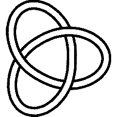
The Coloured Jones Polynomials

KnotTheory`/Navigation  The Mathematica Package KnotTheory` Acknowledgement Setup Naming and Enumeration Presentations Planar Diagrams Some further details Gauss Codes DT (Dowker-Thistlethwaite) Codes Braid Representatives MorseLink Presentations Arc Presentations Conway Notation Graphical Input Graphical Output Drawing Planar Diagrams How does it work? Drawing MorseLink Presentations Drawing Braids Structure and Operations Invariants Invariants from Braid Theory Three Dimensional Invariants The Alexander-Conway Polynomial The Multivariable Alexander Polynomial The Determinant and the Signature The Jones Polynomial How is the Jones polynomial computed? The Coloured Jones Polynomials The A2 Invariant Quantum knot invariants The HOMFLY-PT Polynomial The Kauffman Polynomial Finite Type (Vassiliev) Invariants Khovanov Homology Heegaard Floer Knot Homology R-Matrix Invariants Extras Included with KnotTheory` Drawing with TubePlot Standalone_TubePlot Using the LinKnot package WikiLink QuantumGroups` Lightly Documented Features A Sample KnotTheory` Session Further Usage Example Prime Links with a Non-Prime Component "Rubberband" Brunnian Links Identifying Knots within a List Cabling Burau's Theorem Further Knot Theory Software KnotPlot Knotscape Xknots Extending/Modifying KnotTheory` Bugs How to Edit this Manual...

KnotTheory` can compute the coloured Jones polynomial of knots and links, using the formulas in [Garoufalidis Le]:

(For In[1] see Setup)

In[2]:= ?ColouredJones ColouredJones[K, n][q] returns the coloured Jones polynomial of a knot in colour n (i.e., in the (n 1)-dimensional representation) in the indeterminate q. Some of these polynomials have been precomputed in KnotTheory`. To force computation, use ColouredJones[K,n, Program -> "prog"][q], with "prog" replaced by one of the two available programs, "REngine" or "Braid" (including the quotes). "REngine" (default) computes the invariant for closed knots (as well as links where all components are coloured by the same integer) directly from the MorseLink presentation of the knot, while "Braid" computes the invariant via a presentation of the knot as a braid closure. "REngine" will usually be faster, but it might be better to use "Braid" when (roughly): 1) a "good" braid representative is available for the knot, and 2) the length of this braid is less than the maximum width of the MorseLink presentation of the knot.

In[3]:= ColouredJones::about The "REngine" algorithm was written by Siddarth Sankaran in the summer of 2005, while the "Braid" algorithm was written jointly by Dror Bar-Natan and Stavros Garoufalidis. Both are based on formulas by Thang Le and Stavros Garoufalidis; see [Garoufalidis, S. and Le, T. "The coloured Jones function is q-holonomic." Geom. Top., v9, 2005 (1253-1293)].

Thus, for example, here's the coloured Jones polynomial of the knot 4_1 in the 4-dimensional representation of $sl(2)$:

In[4]:=	ColouredJones[Knot[4, 1], 3][q]
Out[4]=	-12 -11 -10 2 2 3 3 2 4 6 3 q - q - q -- - -- -- - -- - 3 q 3 q - 2 q 8 6 4 2 q q q q 8 10 11 12 2 q - q - q q

And here's the coloured Jones polynomial of the same knot in the two dimensional representation of $sl(2)$; this better be equal to the ordinary Jones polynomial of 4_1!

In[5]:=	ColouredJones[Knot[4, 1], 1][q]
Out[5]=	-2 1 2 1 q - - - q q q

In[6]:=	Jones[Knot[4, 1]][q]
Out[6]=	-2 1 2 1 q - - - q q q

4_1

3_1

In[7]:= ?CJ`Summand CJ`Summand[br, n] returned a pair {s, vars} where s is the summand in the the big sum that makes up ColouredJones[br, n][q] and where vars is the list of variables that need to be summed over (from 0 to n) to get ColouredJones[br, n][q]. CJ`Summand[K, n] is the same for knots for which a braid representative is known to this program.

The coloured Jones polynomial of 3_1 is computed via a single summation. Indeed,

In[8]:=	s = CJ`Summand[Mirror[Knot[3, 1]], n]
Out[8]=	(3 n)/2 n CJ`k[1] (-n 2 CJ`k[1])/2 1 {CJ`q qBinomial[0, 0, ----] CJ`q 1 1 qBinomial[CJ`k[1], 0, ----] qBinomial[CJ`k[1], CJ`k[1], ----] CJ`q CJ`q n 1 n 1 qPochhammer[CJ`q , ----, 0] qPochhammer[CJ`q , ----, CJ`k[1]] CJ`q CJ`q n - CJ`k[1] 1 qPochhammer[CJ`q , ----, 0], {CJ`k[1]}} CJ`q

The symbols in the above formula require a definition:

In[9]:= ?qPochhammer qPochhammer[a, q, k] represents the q-shifted factorial of a in base q with index k. See Eric Weisstein's http://mathworld.wolfram.com/q-PochhammerSymbol.html and Axel Riese's www.risc.uni-linz.ac.at/research/combinat/risc/software/qMultiSum/

In[10]:= ?qBinomial qBinomial[n, k, q] represents the q-binomial coefficient of n and k in base q. For k<0 it is 0; otherwise it is qPochhammer[q^(n-k 1), q, k] / qPochhammer[q, q, k].

More precisely, qPochhammer[a, q, k] is

Failed to parse (unknown function "\begin{cases}"): {\displaystyle (a;q)_k=\begin{cases} (1-a)(1-aq)\dots(1-aq^{k-1})}