The Jones Polynomial

KnotTheory`/Navigation  The Mathematica Package KnotTheory` Acknowledgement Setup Naming and Enumeration Presentations Planar Diagrams Some further details Gauss Codes DT (Dowker-Thistlethwaite) Codes Braid Representatives MorseLink Presentations Arc Presentations Conway Notation Graphical Input Graphical Output Drawing Planar Diagrams How does it work? Drawing MorseLink Presentations Drawing Braids Structure and Operations Invariants Invariants from Braid Theory Three Dimensional Invariants The Alexander-Conway Polynomial The Multivariable Alexander Polynomial The Determinant and the Signature The Jones Polynomial How is the Jones polynomial computed? The Coloured Jones Polynomials The A2 Invariant Quantum knot invariants The HOMFLY-PT Polynomial The Kauffman Polynomial Finite Type (Vassiliev) Invariants Khovanov Homology Heegaard Floer Knot Homology R-Matrix Invariants Extras Included with KnotTheory` Drawing with TubePlot Standalone_TubePlot Using the LinKnot package WikiLink QuantumGroups` Lightly Documented Features A Sample KnotTheory` Session Further Usage Example Prime Links with a Non-Prime Component "Rubberband" Brunnian Links Identifying Knots within a List Cabling Burau's Theorem Further Knot Theory Software KnotPlot Knotscape Xknots Extending/Modifying KnotTheory` Bugs How to Edit this Manual...

(For In[1] see Setup)

Failed to parse (unknown function "\overcrossing"): {\displaystyle a+\overcrossing+1}

In[2]:= ?Jones Jones[L][q] computes the Jones polynomial of a knot or link L as a function of the variable q.

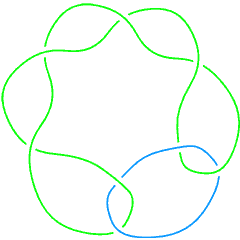
In Naming and Enumeration we checked that the knots 6_1 and 9_46 have the same Alexander polynomial. Their Jones polynomials are different, though:

In[3]:=	Jones[Knot[6, 1]][q]
Out[3]=	-4 -3 -2 2 2 2 + q - q + q - - - q + q q

In[4]:=	Jones[Knot[9, 46]][q]
Out[4]=	-6 -5 -4 2 -2 1 2 + q - q + q - -- + q - - 3 q q

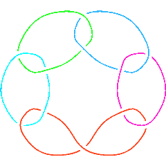
L8a6

On links with an even number of components the Jones polynomial is a function of ${\sqrt {q}}$, and hence it is often more convenient to view it as a function of $t$, where $t^{2}=q$:

In[5]:=	Jones[Link[8, Alternating, 6]][q]
Out[5]=	-(9/2) -(7/2) 3 3 4 3/2 -q + q - ---- + ---- - ------- + 3 Sqrt[q] - 2 q + 5/2 3/2 Sqrt[q] q q 5/2 7/2 2 q - q

In[6]:=	PowerExpand[Jones[Link[8, Alternating, 6]][t^2]]
Out[6]=	-9 -7 3 3 4 3 5 7 -t + t - -- + -- - - + 3 t - 2 t + 2 t - t 5 3 t t t

The Jones polynomial attains 2110 values on the 2226 knots and links known to KnotTheory`:

In[7]:=

all = Join[AllKnots[], AllLinks[]];

In[8]:=	Length /@ {Union[Jones[#][q]& /@ all], all}
Out[8]=	{2110, 2226}

How is the Jones polynomial computed?

(See also: The Kauffman Bracket using Haskell)

The Jones polynomial is so simple to compute using Mathematica that it's worthwhile pause and see how this is done, even for readers with limited prior programming experience. First, recall (say from [Kauffman]) the definition of the Jones polynomial using the Kauffman bracket $\langle \cdot \rangle$:

[KBDef]

Failed to parse (unknown function "\slashoverback"): {\displaystyle \langle\emptyset\rangle=1; \qquad \langle\bigcirc L\rangle = (-A^2-B^2)\langle L\rangle; \qquad \langle\slashoverback\rangle = A\langle\hsmoothing\rangle + B\langle\smoothing\rangle; } $J(L)=\left.(-A^{3})^{w(L)}{\frac {\langle L\rangle }{\langle \bigcirc \rangle }}\right|_{A\to q^{1/4}},$

here $A$ is a commutative variable, $B=A^{-1}$, and $w(L)$ is the writhe of $L$, the difference $n_{+}-n_{-}$ where $n_{+}$ and $n_{-}$ count the positive Failed to parse (unknown function "\overcrossing"): {\displaystyle (\overcrossing)} and negative Failed to parse (SVG (MathML can be enabled via browser plugin): Invalid response ("Math extension cannot connect to Restbase.") from server "https://wikimedia.org/api/rest_v1/":): {\displaystyle (\undercrossing)} crossings of $L$ respectively.

PD[X[1,4,2,5], X[3,6,4,1], X[5,2,6,3]] and P[1,4] P[1,5] P[2,4] P[2,6] P[3,5] P[3,6]

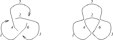
Just for concreteness, let us start by fixing $L$ to be the trefoil knot shown above:

In[9]:=	L = PD[Knot[3, 1]]
Out[9]=	PD[X[1, 4, 2, 5], X[3, 6, 4, 1], X[5, 2, 6, 3]]

Our first task is to perform the replacement Failed to parse (SVG (MathML can be enabled via browser plugin): Invalid response ("Math extension cannot connect to Restbase.") from server "https://wikimedia.org/api/rest_v1/":): {\displaystyle \langle\slashoverback\rangle\to A\langle\hsmoothing\rangle + B\langle\smoothing\rangle} on all crossings of $L$. By our conventions (see Planar Diagrams) the edges around a crossing $X_{abcd}$ are labeled $a$, $b$, $c$ and $d$: Failed to parse (unknown function "\slashoverback"): {\displaystyle {}^c_d\slashoverback{}_a^b} . Labeling the smoothings Failed to parse (unknown function "\hsmoothing"): {\displaystyle (\hsmoothing, \ \smoothing)} in the same way, Failed to parse (unknown function "\hsmoothing"): {\displaystyle {}^c_d\hsmoothing{}_a^b} and Failed to parse (unknown function "\smoothing"): {\displaystyle {}^c_d\smoothing{}_a^b} , we are lead to the symbolic replacement rule $X_{abcd}\to AP_{ad}P_{bc}+BP_{ab}P_{cd}$. Let us apply this rule to $L$, switch to a multiplicative notation and expand:

In[10]:=	t1 = L /. X[a_,b_,c_,d_] :> A P[a,d] P[b,c] + B P[a,b] P[c,d]
Out[10]=	PD[A P[1, 5] P[2, 4] + B P[1, 4] P[2, 5], B P[1, 4] P[3, 6] + A P[1, 3] P[4, 6], A P[2, 6] P[3, 5] + B P[2, 5] P[3, 6]]

In[11]:=

t2 = Expand[Times @@ t1]

Out[11]=

2 A B P[1, 4] P[1, 5] P[2, 4] P[2, 6] P[3, 5] P[3, 6] + 2 2 A B P[1, 4] P[2, 5] P[2, 6] P[3, 5] P[3, 6] + 2 2 A B P[1, 4] P[1, 5] P[2, 4] P[2, 5] P[3, 6] + 3 2 2 2 B P[1, 4] P[2, 5] P[3, 6] + 3 A P[1, 3] P[1, 5] P[2, 4] P[2, 6] P[3, 5] P[4, 6] + 2 A B P[1, 3] P[1, 4] P[2, 5] P[2, 6] P[3, 5] P[4, 6] + 2 A B P[1, 3] P[1, 5] P[2, 4] P[2, 5] P[3, 6] P[4, 6] + 2 2 A B P[1, 3] P[1, 4] P[2, 5] P[3, 6] P[4, 6]

In the above expression the product P[1,4] P[1,5] P[2,4] P[2,6] P[3,5] P[3,6] represents a path in which 1 is connected to 4, 1 is connected to 5, 2 is connected to 4, etc. (see the right half of the figure above). We simplify such paths by repeatedly applying the rules $P_{ab}P_{bc}\to P_{ac}$ and $P_{ab}^{2}\to P_{aa}$:

In[12]:=	t3 = t2 //. {P[a_,b_]P[b_,c_] :> P[a,c], P[a_,b_]^2 :> P[a,a]}
Out[12]=	3 2 B P[1, 1] P[2, 2] P[3, 3] + A B P[2, 2] P[4, 4] + 3 2 2 A P[3, 3] P[4, 4] + A B P[3, 3] P[4, 4] + 3 A B P[5, 5] + 2 A B P[1, 1] P[5, 5]

To complete the computation of the Kauffman bracket, all that remains is to replace closed cycles (paths of the form $P_{aa}$ by $-A^{2}-B^{2}$, to replace $B$ by $A^{-1}$, and to simplify:

In[13]:=	t4 = Expand[t3 /. P[a_,a_] -> -A^2-B^2 /. B -> 1/A]
Out[13]=	-9 1 3 7 -A + - + A + A A

We could have, of course, combined the above four lines to a single very short program, that compues the Kauffman bracket from the beginning to the end:

In[14]:=

KB0[pd_] := Expand[ Expand[Times @@ pd /. X[a_,b_,c_,d_] :> A P[a,d] P[b,c] + 1/A P[a,b] P[c,d]] //. {P[a_,b_]P[b_,c_] :> P[a,c], P[a_,b_]^2 :> P[a,a], P[a_,a_] -> -A^2-1/A^2}]

In[15]:=	t4 = KB0[PD[Knot[3, 1]]]
Out[15]=	-9 1 3 7 -A + - + A + A A

We will skip the uninteresting code for the computation of the writhe here; it is a linear time computation, and if that's all we ever wanted to compute, we wouldn't have bothered to purchase a computer. For our $L$ the result is $-3$, and hence the Jones polynomial of $L$ is given by

In[16]:=	(-A^3)^(-3) * t4 / (-A^2-1/A^2) /. A -> q^(1/4) // Simplify // Expand
Out[16]=	-4 -3 1 -q + q + - q

L11a548

At merely 3 lines of code, our program is surely nice and elegant. But it is very slow:

In[17]:=	time0 = Timing[KB0[PD[Link[11, Alternating, 548]]]]
Out[17]=	-23 5 10 -3 5 13 17 21 25 {1., A + --- + -- + A + 6 A + 6 A + 5 A - 5 A + 4 A - A } 15 7 A A

Here's the much faster alternative employed by KnotTheory`:

In[18]:=

KB1[pd_PD] := KB1[pd, {}, 1]; KB1[pd_PD, inside_, web_] := Module[ {pos = First[Ordering[Length[Complement[List @@ #, inside]]& /@ pd]]}, pd[[pos]] /. X[a_,b_,c_,d_] :> KB1[ Delete[pd, pos], Union[inside, {a,b,c,d}], Expand[web*(A P[a,d] P[b,c]+1/A P[a,b] P[c,d])] //. { P[e_,f_]P[f_,g_] :> P[e,g], P[e_,_]^2 :> P[e,e], P[e_,e_] -> -A^2-1/A^2 } ] ]; KB1[PD[],_,web_] := Expand[web]

In[19]:=	time1 = Timing[KB1[PD[Link[11, Alternating, 548]]]]
Out[19]=	-23 5 10 -3 5 13 17 21 {0.015, A + --- + -- + A + 6 A + 6 A + 5 A - 5 A + 4 A - 15 7 A A 25 A }

(So on L11a548 KB1 is -23 5 10 -3 5 13 17 21 25 {1., A + --- + -- + A + 6 A + 6 A + 5 A - 5 A + 4 A - A }1,1

            15    7
           A     A/         -23    5    10    -3            5      13      17      21    25

{0.015, A + --- + -- + A + 6 A + 6 A + 5 A - 5 A + 4 A - A }1,1

               15    7
              A     A ~              -23    5    10    -3            5      13      17      21    25
      {1., A    + --- + -- + A   + 6 A + 6 A  + 5 A   - 5 A   + 4 A   - A  }1,1
                   15    7
                  A     A

Round[--------------------------------------------------------------------------------]

              -23    5    10    -3            5      13      17      21    25
     {0.015, A    + --- + -- + A   + 6 A + 6 A  + 5 A   - 5 A   + 4 A   - A  }1,1
                     15    7
                    A     A times faster than KB0.)

The idea here is to maintain a "computation front", a planar domain which starts empty and gradualy increases until the whole link diagram is enclosed. Within the front, the rules defining the Kauffman bracket, Equation [KBDef], are applied and the result is expanded as much as possible. Outside of the front the link diagram remains untouched. At every step we choose a crossing outside the front with the most legs inside and "conquer" it -- apply the rules of [KBDef] and expand again. As our new outpost is maximally connected to our old territory, the length of the boundary is increased in a minimal way, and hence the size of the "web" within our front remains as small as possible and thus quick to manipulate.

In further detail, the routine KB1[pd, inside, web] computes the Kauffman bracket assuming the labels of the edges inside the front are in the variable inside, the already-computed inside of the front is in the variable web and the part of the link diagram yet untouched is pd. The single argument KB1[pd] simply calls KB1[pd, inside, web] with an empty inside and with web set to 1. The three argument KB1[pd, inside, web] finds the position of the crossing maximmally connected to the front using the somewhat cryptic assignment

pos = First[Ordering[Length[Complement[List @@ #, inside]]& /@ pd]]}

KB1[pd, inside, web] then recursively calls itself with that crossing removed from pd}, with its legs added to the inside, and with web updated in accordance with [KBDef]. Finally, when pd is empty, the output is simply the value of web.

[Kauffman] ^  L. H. Kauffman, On knots, Princeton Univ. Press, Princeton, 1987.