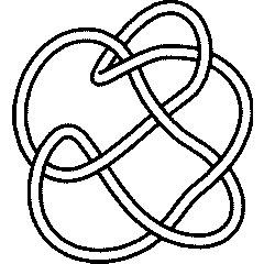
8 15
|
|
|

|
Visit 8 15's page at the Knot Server (KnotPlot driven, includes 3D interactive images!)
Visit 8 15's page at Knotilus! Visit 8 15's page at the original Knot Atlas!
|

Knot presentations
| Planar diagram presentation | X1425 X3849 X5,12,6,13 X13,16,14,1 X9,14,10,15 X15,10,16,11 X11,6,12,7 X7283 |
| Gauss code | -1, 8, -2, 1, -3, 7, -8, 2, -5, 6, -7, 3, -4, 5, -6, 4 |
| Dowker-Thistlethwaite code | 4 8 12 2 14 6 16 10 |
| Conway Notation | [21,21,2] |
|
Length is 9, width is 4. Braid index is 4. |
|
Three dimensional invariants
|
Four dimensional invariants
|
Polynomial invariants
| Alexander polynomial | [math]\displaystyle{ 3 t^2-8 t+11-8 t^{-1} +3 t^{-2} }[/math] |
| Conway polynomial | [math]\displaystyle{ 3 z^4+4 z^2+1 }[/math] |
| 2nd Alexander ideal (db, data sources) | [math]\displaystyle{ \{1\} }[/math] |
| Determinant and Signature | { 33, -4 } |
| Jones polynomial | [math]\displaystyle{ q^{-2} -2 q^{-3} +5 q^{-4} -5 q^{-5} +6 q^{-6} -6 q^{-7} +4 q^{-8} -3 q^{-9} + q^{-10} }[/math] |
| HOMFLY-PT polynomial (db, data sources) | [math]\displaystyle{ a^{10}-3 z^2 a^8-4 a^8+2 z^4 a^6+5 z^2 a^6+3 a^6+z^4 a^4+2 z^2 a^4+a^4 }[/math] |
| Kauffman polynomial (db, data sources) | [math]\displaystyle{ z^4 a^{12}-z^2 a^{12}+3 z^5 a^{11}-5 z^3 a^{11}+2 z a^{11}+3 z^6 a^{10}-3 z^4 a^{10}-a^{10}+z^7 a^9+6 z^5 a^9-14 z^3 a^9+8 z a^9+6 z^6 a^8-10 z^4 a^8+8 z^2 a^8-4 a^8+z^7 a^7+5 z^5 a^7-11 z^3 a^7+6 z a^7+3 z^6 a^6-5 z^4 a^6+5 z^2 a^6-3 a^6+2 z^5 a^5-2 z^3 a^5+z^4 a^4-2 z^2 a^4+a^4 }[/math] |
| The A2 invariant | [math]\displaystyle{ q^{32}+q^{30}-2 q^{28}-q^{26}-2 q^{24}-2 q^{22}+q^{20}+3 q^{16}+q^{14}+q^{12}+2 q^{10}-q^8+q^6 }[/math] |
| The G2 invariant | [math]\displaystyle{ q^{162}-2 q^{160}+4 q^{158}-6 q^{156}+3 q^{154}-q^{152}-6 q^{150}+14 q^{148}-18 q^{146}+20 q^{144}-12 q^{142}-q^{140}+17 q^{138}-27 q^{136}+34 q^{134}-24 q^{132}+7 q^{130}+10 q^{128}-21 q^{126}+25 q^{124}-16 q^{122}+q^{120}+14 q^{118}-20 q^{116}+12 q^{114}-24 q^{110}+34 q^{108}-36 q^{106}+18 q^{104}-2 q^{102}-24 q^{100}+40 q^{98}-47 q^{96}+34 q^{94}-18 q^{92}-7 q^{90}+25 q^{88}-33 q^{86}+26 q^{84}-9 q^{82}-2 q^{80}+16 q^{78}-17 q^{76}+9 q^{74}+10 q^{72}-21 q^{70}+29 q^{68}-21 q^{66}+6 q^{64}+17 q^{62}-27 q^{60}+33 q^{58}-23 q^{56}+12 q^{54}+2 q^{52}-14 q^{50}+17 q^{48}-14 q^{46}+10 q^{44}-2 q^{42}-q^{40}+3 q^{38}-3 q^{36}+3 q^{34}-q^{32}+q^{30} }[/math] |
A1 Invariants.
| Weight | Invariant |
|---|---|
| 1 | [math]\displaystyle{ q^{21}-2 q^{19}+q^{17}-2 q^{15}+q^{11}+3 q^7-q^5+q^3 }[/math] |
| 2 | [math]\displaystyle{ q^{58}-2 q^{56}-2 q^{54}+6 q^{52}-2 q^{50}-6 q^{48}+9 q^{46}+q^{44}-9 q^{42}+6 q^{40}+3 q^{38}-6 q^{36}-q^{34}+2 q^{32}-7 q^{28}+2 q^{26}+7 q^{24}-8 q^{22}+10 q^{18}-5 q^{16}-2 q^{14}+6 q^{12}-q^8+q^6 }[/math] |
| 3 | [math]\displaystyle{ q^{111}-2 q^{109}-2 q^{107}+3 q^{105}+6 q^{103}-2 q^{101}-13 q^{99}+2 q^{97}+18 q^{95}+4 q^{93}-25 q^{91}-13 q^{89}+27 q^{87}+22 q^{85}-27 q^{83}-29 q^{81}+20 q^{79}+35 q^{77}-12 q^{75}-32 q^{73}+7 q^{71}+27 q^{69}+4 q^{67}-21 q^{65}-9 q^{63}+10 q^{61}+17 q^{59}-5 q^{57}-21 q^{55}-7 q^{53}+27 q^{51}+13 q^{49}-30 q^{47}-23 q^{45}+27 q^{43}+27 q^{41}-22 q^{39}-32 q^{37}+12 q^{35}+32 q^{33}-6 q^{31}-23 q^{29}-2 q^{27}+19 q^{25}+7 q^{23}-8 q^{21}-4 q^{19}+4 q^{17}+3 q^{15}-q^{11}+q^9 }[/math] |
| 4 | [math]\displaystyle{ q^{180}-2 q^{178}-2 q^{176}+3 q^{174}+3 q^{172}+6 q^{170}-9 q^{168}-13 q^{166}+2 q^{164}+11 q^{162}+30 q^{160}-11 q^{158}-41 q^{156}-22 q^{154}+14 q^{152}+80 q^{150}+22 q^{148}-62 q^{146}-83 q^{144}-27 q^{142}+123 q^{140}+97 q^{138}-31 q^{136}-135 q^{134}-108 q^{132}+102 q^{130}+151 q^{128}+41 q^{126}-124 q^{124}-159 q^{122}+38 q^{120}+138 q^{118}+88 q^{116}-63 q^{114}-137 q^{112}-19 q^{110}+80 q^{108}+92 q^{106}-2 q^{104}-81 q^{102}-57 q^{100}+17 q^{98}+75 q^{96}+49 q^{94}-23 q^{92}-93 q^{90}-46 q^{88}+62 q^{86}+102 q^{84}+34 q^{82}-121 q^{80}-107 q^{78}+32 q^{76}+141 q^{74}+101 q^{72}-112 q^{70}-148 q^{68}-28 q^{66}+124 q^{64}+148 q^{62}-49 q^{60}-133 q^{58}-86 q^{56}+53 q^{54}+136 q^{52}+19 q^{50}-62 q^{48}-83 q^{46}-12 q^{44}+70 q^{42}+38 q^{40}-38 q^{36}-24 q^{34}+16 q^{32}+14 q^{30}+11 q^{28}-5 q^{26}-7 q^{24}+2 q^{22}+q^{20}+3 q^{18}-q^{14}+q^{12} }[/math] |
| 5 | [math]\displaystyle{ q^{265}-2 q^{263}-2 q^{261}+3 q^{259}+3 q^{257}+3 q^{255}-q^{253}-9 q^{251}-13 q^{249}+2 q^{247}+20 q^{245}+23 q^{243}+6 q^{241}-27 q^{239}-49 q^{237}-33 q^{235}+37 q^{233}+92 q^{231}+71 q^{229}-21 q^{227}-131 q^{225}-155 q^{223}-29 q^{221}+172 q^{219}+255 q^{217}+121 q^{215}-157 q^{213}-369 q^{211}-275 q^{209}+93 q^{207}+447 q^{205}+449 q^{203}+42 q^{201}-464 q^{199}-612 q^{197}-218 q^{195}+403 q^{193}+725 q^{191}+409 q^{189}-288 q^{187}-747 q^{185}-557 q^{183}+129 q^{181}+696 q^{179}+645 q^{177}+23 q^{175}-589 q^{173}-647 q^{171}-147 q^{169}+441 q^{167}+591 q^{165}+229 q^{163}-299 q^{161}-511 q^{159}-260 q^{157}+162 q^{155}+395 q^{153}+289 q^{151}-49 q^{149}-310 q^{147}-287 q^{145}-48 q^{143}+215 q^{141}+319 q^{139}+152 q^{137}-156 q^{135}-340 q^{133}-254 q^{131}+77 q^{129}+394 q^{127}+373 q^{125}-7 q^{123}-426 q^{121}-499 q^{119}-98 q^{117}+448 q^{115}+620 q^{113}+214 q^{111}-413 q^{109}-712 q^{107}-360 q^{105}+339 q^{103}+747 q^{101}+494 q^{99}-202 q^{97}-709 q^{95}-595 q^{93}+27 q^{91}+607 q^{89}+634 q^{87}+132 q^{85}-435 q^{83}-592 q^{81}-272 q^{79}+239 q^{77}+496 q^{75}+313 q^{73}-70 q^{71}-337 q^{69}-309 q^{67}-55 q^{65}+194 q^{63}+240 q^{61}+101 q^{59}-72 q^{57}-154 q^{55}-101 q^{53}+6 q^{51}+77 q^{49}+74 q^{47}+18 q^{45}-27 q^{43}-36 q^{41}-14 q^{39}+4 q^{37}+17 q^{35}+12 q^{33}-q^{31}-4 q^{29}-q^{27}-q^{25}+q^{23}+3 q^{21}-q^{17}+q^{15} }[/math] |
A2 Invariants.
| Weight | Invariant |
|---|---|
| 1,0 | [math]\displaystyle{ q^{32}+q^{30}-2 q^{28}-q^{26}-2 q^{24}-2 q^{22}+q^{20}+3 q^{16}+q^{14}+q^{12}+2 q^{10}-q^8+q^6 }[/math] |
| 1,1 | [math]\displaystyle{ q^{84}-4 q^{82}+10 q^{80}-20 q^{78}+34 q^{76}-54 q^{74}+74 q^{72}-92 q^{70}+105 q^{68}-104 q^{66}+90 q^{64}-60 q^{62}+18 q^{60}+36 q^{58}-90 q^{56}+142 q^{54}-176 q^{52}+200 q^{50}-202 q^{48}+182 q^{46}-153 q^{44}+96 q^{42}-52 q^{40}-10 q^{38}+48 q^{36}-86 q^{34}+104 q^{32}-104 q^{30}+99 q^{28}-72 q^{26}+62 q^{24}-34 q^{22}+25 q^{20}-10 q^{18}+6 q^{16}-2 q^{14}+q^{12} }[/math] |
| 2,0 | [math]\displaystyle{ q^{80}+q^{78}-q^{76}-4 q^{74}-3 q^{72}+2 q^{70}+q^{68}+3 q^{64}+8 q^{62}+4 q^{60}-3 q^{58}+2 q^{54}-4 q^{52}-6 q^{50}-3 q^{48}-3 q^{46}-6 q^{44}-2 q^{42}+q^{40}-3 q^{38}+6 q^{34}+3 q^{32}-3 q^{30}+4 q^{28}+6 q^{26}+q^{24}-2 q^{22}+3 q^{20}+4 q^{18}-q^{16}-q^{14}+q^{12} }[/math] |
A3 Invariants.
| Weight | Invariant |
|---|---|
| 0,1,0 | [math]\displaystyle{ q^{68}-2 q^{66}+3 q^{62}-6 q^{60}+q^{58}+6 q^{56}-5 q^{54}+4 q^{52}+10 q^{50}-3 q^{48}-q^{46}-q^{44}-7 q^{42}-9 q^{40}-7 q^{38}+q^{36}-q^{34}-2 q^{32}+10 q^{30}+5 q^{28}-4 q^{26}+9 q^{24}+2 q^{22}-3 q^{20}+4 q^{18}+q^{16}-q^{14}+q^{12} }[/math] |
| 1,0,0 | [math]\displaystyle{ q^{43}+q^{41}+q^{39}-2 q^{37}-q^{35}-4 q^{33}-2 q^{31}-2 q^{29}+q^{27}+q^{25}+2 q^{23}+3 q^{21}+q^{19}+2 q^{17}+2 q^{13}-q^{11}+q^9 }[/math] |
A4 Invariants.
| Weight | Invariant |
|---|---|
| 0,1,0,0 | [math]\displaystyle{ q^{90}+q^{88}-q^{86}-3 q^{84}-q^{82}-5 q^{78}-4 q^{76}+6 q^{74}+8 q^{72}+3 q^{70}+9 q^{68}+14 q^{66}+5 q^{64}-5 q^{62}-4 q^{60}-9 q^{58}-20 q^{56}-17 q^{54}-7 q^{52}-10 q^{50}-6 q^{48}+9 q^{46}+9 q^{44}+2 q^{42}+7 q^{40}+12 q^{38}+4 q^{36}-q^{34}+4 q^{32}+6 q^{30}-q^{28}+3 q^{24}+q^{22}-q^{20}+q^{18} }[/math] |
| 1,0,0,0 | [math]\displaystyle{ q^{54}+q^{52}+q^{50}+q^{48}-2 q^{46}-q^{44}-4 q^{42}-4 q^{40}-2 q^{38}-2 q^{36}+q^{34}+q^{32}+3 q^{30}+2 q^{28}+3 q^{26}+q^{24}+2 q^{22}+q^{20}+2 q^{16}-q^{14}+q^{12} }[/math] |
B2 Invariants.
| Weight | Invariant |
|---|---|
| 0,1 | [math]\displaystyle{ q^{68}-2 q^{66}+4 q^{64}-5 q^{62}+6 q^{60}-7 q^{58}+6 q^{56}-5 q^{54}+2 q^{52}-5 q^{48}+7 q^{46}-11 q^{44}+11 q^{42}-13 q^{40}+11 q^{38}-9 q^{36}+7 q^{34}-2 q^{32}+5 q^{28}-4 q^{26}+7 q^{24}-6 q^{22}+7 q^{20}-4 q^{18}+3 q^{16}-q^{14}+q^{12} }[/math] |
| 1,0 | [math]\displaystyle{ q^{110}-2 q^{106}-2 q^{104}+2 q^{102}+4 q^{100}-q^{98}-6 q^{96}-3 q^{94}+6 q^{92}+6 q^{90}-2 q^{88}-6 q^{86}+q^{84}+8 q^{82}+5 q^{80}-4 q^{78}-3 q^{76}+3 q^{74}+3 q^{72}-5 q^{70}-7 q^{68}-2 q^{66}+2 q^{64}-3 q^{62}-7 q^{60}-3 q^{58}+3 q^{56}+3 q^{54}-4 q^{52}-3 q^{50}+5 q^{48}+9 q^{46}-5 q^{42}-q^{40}+8 q^{38}+6 q^{36}-2 q^{34}-5 q^{32}+q^{30}+4 q^{28}+2 q^{26}-q^{24}-q^{22}+q^{18} }[/math] |
D4 Invariants.
| Weight | Invariant |
|---|---|
| 1,0,0,0 | [math]\displaystyle{ q^{94}-2 q^{92}+2 q^{90}-3 q^{88}+4 q^{86}-6 q^{84}+4 q^{82}-5 q^{80}+6 q^{78}-3 q^{76}+4 q^{74}+2 q^{72}+5 q^{70}+6 q^{68}-4 q^{66}+5 q^{64}-10 q^{62}+4 q^{60}-17 q^{58}-16 q^{54}+4 q^{52}-8 q^{50}+5 q^{48}-2 q^{46}+6 q^{44}+7 q^{42}+2 q^{40}+6 q^{38}-2 q^{36}+8 q^{34}-3 q^{32}+6 q^{30}-4 q^{28}+5 q^{26}-q^{24}+2 q^{22}-q^{20}+q^{18} }[/math] |
G2 Invariants.
| Weight | Invariant |
|---|---|
| 1,0 | [math]\displaystyle{ q^{162}-2 q^{160}+4 q^{158}-6 q^{156}+3 q^{154}-q^{152}-6 q^{150}+14 q^{148}-18 q^{146}+20 q^{144}-12 q^{142}-q^{140}+17 q^{138}-27 q^{136}+34 q^{134}-24 q^{132}+7 q^{130}+10 q^{128}-21 q^{126}+25 q^{124}-16 q^{122}+q^{120}+14 q^{118}-20 q^{116}+12 q^{114}-24 q^{110}+34 q^{108}-36 q^{106}+18 q^{104}-2 q^{102}-24 q^{100}+40 q^{98}-47 q^{96}+34 q^{94}-18 q^{92}-7 q^{90}+25 q^{88}-33 q^{86}+26 q^{84}-9 q^{82}-2 q^{80}+16 q^{78}-17 q^{76}+9 q^{74}+10 q^{72}-21 q^{70}+29 q^{68}-21 q^{66}+6 q^{64}+17 q^{62}-27 q^{60}+33 q^{58}-23 q^{56}+12 q^{54}+2 q^{52}-14 q^{50}+17 q^{48}-14 q^{46}+10 q^{44}-2 q^{42}-q^{40}+3 q^{38}-3 q^{36}+3 q^{34}-q^{32}+q^{30} }[/math] |
.
KnotTheory`, as shown in the (simulated) Mathematica session below. Your input (in red) is realistic; all else should have the same content as in a real mathematica session, but with different formatting. This Mathematica session is also available (albeit only for the knot 5_2) as the notebook PolynomialInvariantsSession.nb.
(The path below may be different on your system, and possibly also the KnotTheory` date)
In[1]:=
|
AppendTo[$Path, "C:/drorbn/projects/KAtlas/"];
<< KnotTheory`
|
Loading KnotTheory` version of August 31, 2006, 11:25:27.5625.
|
In[3]:=
|
K = Knot["8 15"];
|
In[4]:=
|
Alexander[K][t]
|
KnotTheory::loading: Loading precomputed data in PD4Knots`.
|
Out[4]=
|
[math]\displaystyle{ 3 t^2-8 t+11-8 t^{-1} +3 t^{-2} }[/math] |
In[5]:=
|
Conway[K][z]
|
Out[5]=
|
[math]\displaystyle{ 3 z^4+4 z^2+1 }[/math] |
In[6]:=
|
Alexander[K, 2][t]
|
KnotTheory::credits: The program Alexander[K, r] to compute Alexander ideals was written by Jana Archibald at the University of Toronto in the summer of 2005.
|
Out[6]=
|
[math]\displaystyle{ \{1\} }[/math] |
In[7]:=
|
{KnotDet[K], KnotSignature[K]}
|
Out[7]=
|
{ 33, -4 } |
In[8]:=
|
Jones[K][q]
|
KnotTheory::loading: Loading precomputed data in Jones4Knots`.
|
Out[8]=
|
[math]\displaystyle{ q^{-2} -2 q^{-3} +5 q^{-4} -5 q^{-5} +6 q^{-6} -6 q^{-7} +4 q^{-8} -3 q^{-9} + q^{-10} }[/math] |
In[9]:=
|
HOMFLYPT[K][a, z]
|
KnotTheory::credits: The HOMFLYPT program was written by Scott Morrison.
|
Out[9]=
|
[math]\displaystyle{ a^{10}-3 z^2 a^8-4 a^8+2 z^4 a^6+5 z^2 a^6+3 a^6+z^4 a^4+2 z^2 a^4+a^4 }[/math] |
In[10]:=
|
Kauffman[K][a, z]
|
KnotTheory::loading: Loading precomputed data in Kauffman4Knots`.
|
Out[10]=
|
[math]\displaystyle{ z^4 a^{12}-z^2 a^{12}+3 z^5 a^{11}-5 z^3 a^{11}+2 z a^{11}+3 z^6 a^{10}-3 z^4 a^{10}-a^{10}+z^7 a^9+6 z^5 a^9-14 z^3 a^9+8 z a^9+6 z^6 a^8-10 z^4 a^8+8 z^2 a^8-4 a^8+z^7 a^7+5 z^5 a^7-11 z^3 a^7+6 z a^7+3 z^6 a^6-5 z^4 a^6+5 z^2 a^6-3 a^6+2 z^5 a^5-2 z^3 a^5+z^4 a^4-2 z^2 a^4+a^4 }[/math] |
"Similar" Knots (within the Atlas)
Same Alexander/Conway Polynomial: {K11n65, ...}
Same Jones Polynomial (up to mirroring, [math]\displaystyle{ q\leftrightarrow q^{-1} }[/math]): {...}
Vassiliev invariants
| V2 and V3: | (4, -7) |
| V2,1 through V6,9: |
|
V2,1 through V6,9 were provided by Petr Dunin-Barkowski <barkovs@itep.ru>, Andrey Smirnov <asmirnov@itep.ru>, and Alexei Sleptsov <sleptsov@itep.ru> and uploaded on October 2010 by User:Drorbn. Note that they are normalized differently than V2 and V3.
Khovanov Homology
| The coefficients of the monomials [math]\displaystyle{ t^rq^j }[/math] are shown, along with their alternating sums [math]\displaystyle{ \chi }[/math] (fixed [math]\displaystyle{ j }[/math], alternation over [math]\displaystyle{ r }[/math]). The squares with yellow highlighting are those on the "critical diagonals", where [math]\displaystyle{ j-2r=s+1 }[/math] or [math]\displaystyle{ j-2r=s-1 }[/math], where [math]\displaystyle{ s= }[/math]-4 is the signature of 8 15. Nonzero entries off the critical diagonals (if any exist) are highlighted in red. |
|
| Integral Khovanov Homology
(db, data source) |
|
The Coloured Jones Polynomials
| [math]\displaystyle{ n }[/math] | [math]\displaystyle{ J_n }[/math] |
| 2 | [math]\displaystyle{ q^{-4} -2 q^{-5} + q^{-6} +7 q^{-7} -10 q^{-8} -2 q^{-9} +22 q^{-10} -20 q^{-11} -10 q^{-12} +37 q^{-13} -25 q^{-14} -19 q^{-15} +44 q^{-16} -23 q^{-17} -22 q^{-18} +39 q^{-19} -14 q^{-20} -19 q^{-21} +24 q^{-22} -4 q^{-23} -11 q^{-24} +9 q^{-25} -3 q^{-27} + q^{-28} }[/math] |
| 3 | [math]\displaystyle{ q^{-6} -2 q^{-7} + q^{-8} +3 q^{-9} +2 q^{-10} -10 q^{-11} -3 q^{-12} +18 q^{-13} +14 q^{-14} -31 q^{-15} -24 q^{-16} +35 q^{-17} +52 q^{-18} -51 q^{-19} -68 q^{-20} +45 q^{-21} +101 q^{-22} -51 q^{-23} -118 q^{-24} +38 q^{-25} +144 q^{-26} -37 q^{-27} -152 q^{-28} +24 q^{-29} +160 q^{-30} -15 q^{-31} -159 q^{-32} +5 q^{-33} +148 q^{-34} +10 q^{-35} -136 q^{-36} -15 q^{-37} +109 q^{-38} +30 q^{-39} -89 q^{-40} -30 q^{-41} +60 q^{-42} +32 q^{-43} -40 q^{-44} -25 q^{-45} +20 q^{-46} +20 q^{-47} -11 q^{-48} -11 q^{-49} +4 q^{-50} +5 q^{-51} -3 q^{-53} + q^{-54} }[/math] |
| 4 | [math]\displaystyle{ q^{-8} -2 q^{-9} + q^{-10} +3 q^{-11} -2 q^{-12} +2 q^{-13} -11 q^{-14} +3 q^{-15} +19 q^{-16} + q^{-17} +4 q^{-18} -51 q^{-19} -11 q^{-20} +57 q^{-21} +39 q^{-22} +36 q^{-23} -133 q^{-24} -82 q^{-25} +78 q^{-26} +120 q^{-27} +153 q^{-28} -216 q^{-29} -221 q^{-30} +31 q^{-31} +204 q^{-32} +350 q^{-33} -240 q^{-34} -373 q^{-35} -89 q^{-36} +240 q^{-37} +563 q^{-38} -200 q^{-39} -482 q^{-40} -228 q^{-41} +226 q^{-42} +718 q^{-43} -132 q^{-44} -522 q^{-45} -336 q^{-46} +179 q^{-47} +788 q^{-48} -60 q^{-49} -496 q^{-50} -394 q^{-51} +105 q^{-52} +764 q^{-53} +19 q^{-54} -402 q^{-55} -406 q^{-56} +6 q^{-57} +646 q^{-58} +93 q^{-59} -251 q^{-60} -356 q^{-61} -94 q^{-62} +449 q^{-63} +128 q^{-64} -86 q^{-65} -246 q^{-66} -143 q^{-67} +239 q^{-68} +101 q^{-69} +18 q^{-70} -118 q^{-71} -117 q^{-72} +89 q^{-73} +45 q^{-74} +39 q^{-75} -34 q^{-76} -59 q^{-77} +23 q^{-78} +9 q^{-79} +20 q^{-80} -4 q^{-81} -18 q^{-82} +4 q^{-83} +5 q^{-85} -3 q^{-87} + q^{-88} }[/math] |
| 5 | [math]\displaystyle{ q^{-10} -2 q^{-11} + q^{-12} +3 q^{-13} -2 q^{-14} -2 q^{-15} + q^{-16} -5 q^{-17} +4 q^{-18} +16 q^{-19} +3 q^{-20} -15 q^{-21} -17 q^{-22} -27 q^{-23} +13 q^{-24} +61 q^{-25} +59 q^{-26} -12 q^{-27} -88 q^{-28} -134 q^{-29} -40 q^{-30} +143 q^{-31} +232 q^{-32} +127 q^{-33} -134 q^{-34} -383 q^{-35} -294 q^{-36} +115 q^{-37} +499 q^{-38} +510 q^{-39} +49 q^{-40} -640 q^{-41} -805 q^{-42} -205 q^{-43} +656 q^{-44} +1077 q^{-45} +551 q^{-46} -667 q^{-47} -1385 q^{-48} -827 q^{-49} +542 q^{-50} +1584 q^{-51} +1247 q^{-52} -414 q^{-53} -1793 q^{-54} -1526 q^{-55} +190 q^{-56} +1883 q^{-57} +1874 q^{-58} -8 q^{-59} -1965 q^{-60} -2072 q^{-61} -211 q^{-62} +1956 q^{-63} +2293 q^{-64} +372 q^{-65} -1944 q^{-66} -2389 q^{-67} -542 q^{-68} +1870 q^{-69} +2477 q^{-70} +680 q^{-71} -1777 q^{-72} -2493 q^{-73} -805 q^{-74} +1631 q^{-75} +2454 q^{-76} +941 q^{-77} -1439 q^{-78} -2387 q^{-79} -1038 q^{-80} +1209 q^{-81} +2203 q^{-82} +1153 q^{-83} -911 q^{-84} -2025 q^{-85} -1188 q^{-86} +621 q^{-87} +1703 q^{-88} +1211 q^{-89} -299 q^{-90} -1403 q^{-91} -1137 q^{-92} +54 q^{-93} +1017 q^{-94} +1021 q^{-95} +160 q^{-96} -706 q^{-97} -821 q^{-98} -268 q^{-99} +396 q^{-100} +627 q^{-101} +308 q^{-102} -200 q^{-103} -414 q^{-104} -270 q^{-105} +42 q^{-106} +259 q^{-107} +214 q^{-108} +12 q^{-109} -136 q^{-110} -136 q^{-111} -41 q^{-112} +58 q^{-113} +88 q^{-114} +36 q^{-115} -26 q^{-116} -44 q^{-117} -20 q^{-118} +3 q^{-119} +18 q^{-120} +20 q^{-121} -4 q^{-122} -11 q^{-123} -3 q^{-124} +5 q^{-127} -3 q^{-129} + q^{-130} }[/math] |
| 6 | [math]\displaystyle{ q^{-12} -2 q^{-13} + q^{-14} +3 q^{-15} -2 q^{-16} -2 q^{-17} -3 q^{-18} +7 q^{-19} -4 q^{-20} + q^{-21} +18 q^{-22} -6 q^{-23} -14 q^{-24} -25 q^{-25} +9 q^{-26} -4 q^{-27} +20 q^{-28} +82 q^{-29} +17 q^{-30} -42 q^{-31} -124 q^{-32} -60 q^{-33} -73 q^{-34} +60 q^{-35} +299 q^{-36} +216 q^{-37} +49 q^{-38} -301 q^{-39} -346 q^{-40} -472 q^{-41} -113 q^{-42} +618 q^{-43} +804 q^{-44} +644 q^{-45} -179 q^{-46} -714 q^{-47} -1468 q^{-48} -1020 q^{-49} +496 q^{-50} +1564 q^{-51} +2011 q^{-52} +879 q^{-53} -459 q^{-54} -2719 q^{-55} -2904 q^{-56} -790 q^{-57} +1677 q^{-58} +3681 q^{-59} +3049 q^{-60} +1117 q^{-61} -3312 q^{-62} -5153 q^{-63} -3295 q^{-64} +491 q^{-65} +4699 q^{-66} +5613 q^{-67} +3891 q^{-68} -2673 q^{-69} -6793 q^{-70} -6189 q^{-71} -1759 q^{-72} +4584 q^{-73} +7623 q^{-74} +6936 q^{-75} -1104 q^{-76} -7386 q^{-77} -8535 q^{-78} -4188 q^{-79} +3648 q^{-80} +8682 q^{-81} +9364 q^{-82} +622 q^{-83} -7176 q^{-84} -9954 q^{-85} -6082 q^{-86} +2500 q^{-87} +8961 q^{-88} +10872 q^{-89} +1999 q^{-90} -6597 q^{-91} -10565 q^{-92} -7282 q^{-93} +1444 q^{-94} +8747 q^{-95} +11598 q^{-96} +3029 q^{-97} -5800 q^{-98} -10582 q^{-99} -7983 q^{-100} +381 q^{-101} +8084 q^{-102} +11714 q^{-103} +3946 q^{-104} -4607 q^{-105} -9983 q^{-106} -8338 q^{-107} -922 q^{-108} +6758 q^{-109} +11131 q^{-110} +4841 q^{-111} -2802 q^{-112} -8521 q^{-113} -8179 q^{-114} -2448 q^{-115} +4601 q^{-116} +9567 q^{-117} +5393 q^{-118} -556 q^{-119} -6075 q^{-120} -7120 q^{-121} -3682 q^{-122} +1937 q^{-123} +6946 q^{-124} +5054 q^{-125} +1386 q^{-126} -3121 q^{-127} -5044 q^{-128} -3915 q^{-129} -317 q^{-130} +3866 q^{-131} +3649 q^{-132} +2197 q^{-133} -685 q^{-134} -2574 q^{-135} -2977 q^{-136} -1340 q^{-137} +1399 q^{-138} +1826 q^{-139} +1782 q^{-140} +478 q^{-141} -716 q^{-142} -1572 q^{-143} -1173 q^{-144} +170 q^{-145} +506 q^{-146} +898 q^{-147} +546 q^{-148} +87 q^{-149} -552 q^{-150} -592 q^{-151} -98 q^{-152} -17 q^{-153} +280 q^{-154} +257 q^{-155} +183 q^{-156} -121 q^{-157} -198 q^{-158} -47 q^{-159} -74 q^{-160} +47 q^{-161} +69 q^{-162} +91 q^{-163} -18 q^{-164} -47 q^{-165} -5 q^{-166} -31 q^{-167} +3 q^{-168} +9 q^{-169} +29 q^{-170} -4 q^{-171} -11 q^{-172} +4 q^{-173} -7 q^{-174} +5 q^{-177} -3 q^{-179} + q^{-180} }[/math] |
| 7 | [math]\displaystyle{ q^{-14} -2 q^{-15} + q^{-16} +3 q^{-17} -2 q^{-18} -2 q^{-19} -3 q^{-20} +3 q^{-21} +8 q^{-22} -7 q^{-23} +3 q^{-24} +9 q^{-25} -5 q^{-26} -12 q^{-27} -22 q^{-28} +35 q^{-30} +4 q^{-31} +29 q^{-32} +35 q^{-33} -13 q^{-34} -53 q^{-35} -126 q^{-36} -76 q^{-37} +47 q^{-38} +77 q^{-39} +199 q^{-40} +233 q^{-41} +88 q^{-42} -100 q^{-43} -440 q^{-44} -525 q^{-45} -273 q^{-46} -5 q^{-47} +593 q^{-48} +972 q^{-49} +869 q^{-50} +389 q^{-51} -720 q^{-52} -1582 q^{-53} -1698 q^{-54} -1248 q^{-55} +377 q^{-56} +2113 q^{-57} +2971 q^{-58} +2752 q^{-59} +538 q^{-60} -2251 q^{-61} -4283 q^{-62} -4961 q^{-63} -2506 q^{-64} +1649 q^{-65} +5479 q^{-66} +7594 q^{-67} +5418 q^{-68} +195 q^{-69} -5775 q^{-70} -10470 q^{-71} -9460 q^{-72} -3321 q^{-73} +5123 q^{-74} +12813 q^{-75} +13835 q^{-76} +7927 q^{-77} -2683 q^{-78} -14330 q^{-79} -18648 q^{-80} -13455 q^{-81} -932 q^{-82} +14463 q^{-83} +22554 q^{-84} +19601 q^{-85} +6291 q^{-86} -13197 q^{-87} -25969 q^{-88} -25701 q^{-89} -12026 q^{-90} +10580 q^{-91} +27728 q^{-92} +31256 q^{-93} +18529 q^{-94} -6954 q^{-95} -28747 q^{-96} -35892 q^{-97} -24396 q^{-98} +2813 q^{-99} +28289 q^{-100} +39474 q^{-101} +30019 q^{-102} +1428 q^{-103} -27450 q^{-104} -41993 q^{-105} -34422 q^{-106} -5428 q^{-107} +25855 q^{-108} +43610 q^{-109} +38187 q^{-110} +8921 q^{-111} -24374 q^{-112} -44475 q^{-113} -40815 q^{-114} -11853 q^{-115} +22629 q^{-116} +44836 q^{-117} +42923 q^{-118} +14253 q^{-119} -21172 q^{-120} -44808 q^{-121} -44255 q^{-122} -16241 q^{-123} +19570 q^{-124} +44457 q^{-125} +45310 q^{-126} +18010 q^{-127} -18022 q^{-128} -43820 q^{-129} -45938 q^{-130} -19653 q^{-131} +16181 q^{-132} +42728 q^{-133} +46276 q^{-134} +21395 q^{-135} -13920 q^{-136} -41152 q^{-137} -46293 q^{-138} -23147 q^{-139} +11205 q^{-140} +38759 q^{-141} +45645 q^{-142} +25027 q^{-143} -7705 q^{-144} -35542 q^{-145} -44468 q^{-146} -26695 q^{-147} +3879 q^{-148} +31235 q^{-149} +42093 q^{-150} +28009 q^{-151} +598 q^{-152} -26035 q^{-153} -38856 q^{-154} -28555 q^{-155} -4784 q^{-156} +20059 q^{-157} +34166 q^{-158} +28072 q^{-159} +8765 q^{-160} -13734 q^{-161} -28722 q^{-162} -26344 q^{-163} -11572 q^{-164} +7629 q^{-165} +22422 q^{-166} +23332 q^{-167} +13290 q^{-168} -2311 q^{-169} -16171 q^{-170} -19357 q^{-171} -13373 q^{-172} -1746 q^{-173} +10239 q^{-174} +14864 q^{-175} +12281 q^{-176} +4278 q^{-177} -5489 q^{-178} -10336 q^{-179} -10095 q^{-180} -5371 q^{-181} +1885 q^{-182} +6422 q^{-183} +7634 q^{-184} +5202 q^{-185} +204 q^{-186} -3350 q^{-187} -5056 q^{-188} -4347 q^{-189} -1288 q^{-190} +1312 q^{-191} +3053 q^{-192} +3187 q^{-193} +1417 q^{-194} -167 q^{-195} -1526 q^{-196} -2043 q^{-197} -1225 q^{-198} -356 q^{-199} +639 q^{-200} +1216 q^{-201} +838 q^{-202} +408 q^{-203} -166 q^{-204} -603 q^{-205} -476 q^{-206} -375 q^{-207} -46 q^{-208} +307 q^{-209} +268 q^{-210} +227 q^{-211} +52 q^{-212} -117 q^{-213} -89 q^{-214} -137 q^{-215} -85 q^{-216} +50 q^{-217} +59 q^{-218} +72 q^{-219} +26 q^{-220} -28 q^{-221} +3 q^{-222} -27 q^{-223} -31 q^{-224} +3 q^{-225} +9 q^{-226} +20 q^{-227} +5 q^{-228} -11 q^{-229} +4 q^{-230} -7 q^{-232} +5 q^{-235} -3 q^{-237} + q^{-238} }[/math] |
Computer Talk
Much of the above data can be recomputed by Mathematica using the package KnotTheory`. See A Sample KnotTheory` Session.
In[1]:= |
<< KnotTheory` |
Loading KnotTheory` (version of August 29, 2005, 15:27:48)... | |
In[2]:= | PD[Knot[8, 15]] |
Out[2]= | PD[X[1, 4, 2, 5], X[3, 8, 4, 9], X[5, 12, 6, 13], X[13, 16, 14, 1], X[9, 14, 10, 15], X[15, 10, 16, 11], X[11, 6, 12, 7], X[7, 2, 8, 3]] |
In[3]:= | GaussCode[Knot[8, 15]] |
Out[3]= | GaussCode[-1, 8, -2, 1, -3, 7, -8, 2, -5, 6, -7, 3, -4, 5, -6, 4] |
In[4]:= | DTCode[Knot[8, 15]] |
Out[4]= | DTCode[4, 8, 12, 2, 14, 6, 16, 10] |
In[5]:= | br = BR[Knot[8, 15]] |
Out[5]= | BR[4, {-1, -1, 2, -1, -3, -2, -2, -2, -3}] |
In[6]:= | {First[br], Crossings[br]} |
Out[6]= | {4, 9} |
In[7]:= | BraidIndex[Knot[8, 15]] |
Out[7]= | 4 |
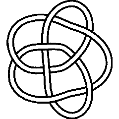
In[8]:= | Show[DrawMorseLink[Knot[8, 15]]] |
 | |
| Out[8]= | -Graphics- |
In[9]:= | (#[Knot[8, 15]]&) /@ {SymmetryType, UnknottingNumber, ThreeGenus, BridgeIndex, SuperBridgeIndex, NakanishiIndex} |
Out[9]= | {Reversible, 2, 2, 3, {4, 6}, 1} |
In[10]:= | alex = Alexander[Knot[8, 15]][t] |
Out[10]= | 3 8 2 |
In[11]:= | Conway[Knot[8, 15]][z] |
Out[11]= | 2 4 1 + 4 z + 3 z |
In[12]:= | Select[AllKnots[], (alex === Alexander[#][t])&] |
Out[12]= | {Knot[8, 15], Knot[11, NonAlternating, 65]} |
In[13]:= | {KnotDet[Knot[8, 15]], KnotSignature[Knot[8, 15]]} |
Out[13]= | {33, -4} |
In[14]:= | Jones[Knot[8, 15]][q] |
Out[14]= | -10 3 4 6 6 5 5 2 -2 |
In[15]:= | Select[AllKnots[], (J === Jones[#][q] || (J /. q-> 1/q) === Jones[#][q])&] |
Out[15]= | {Knot[8, 15]} |
In[16]:= | A2Invariant[Knot[8, 15]][q] |
Out[16]= | -32 -30 2 -26 2 2 -20 3 -14 -12 2 |
In[17]:= | HOMFLYPT[Knot[8, 15]][a, z] |
Out[17]= | 4 6 8 10 4 2 6 2 8 2 4 4 6 4 a + 3 a - 4 a + a + 2 a z + 5 a z - 3 a z + a z + 2 a z |
In[18]:= | Kauffman[Knot[8, 15]][a, z] |
Out[18]= | 4 6 8 10 7 9 11 4 2 |
In[19]:= | {Vassiliev[2][Knot[8, 15]], Vassiliev[3][Knot[8, 15]]} |
Out[19]= | {4, -7} |
In[20]:= | Kh[Knot[8, 15]][q, t] |
Out[20]= | -5 -3 1 2 1 2 2 4 |
In[21]:= | ColouredJones[Knot[8, 15], 2][q] |
Out[21]= | -28 3 9 11 4 24 19 14 39 22 23 |
| See/edit the Rolfsen_Splice_Template.
Back to the top. |
|