L2a1

L2a1

L4a1

	Visit L2a1's page at Knotilus! Visit L2a1's page at the original Knot Atlas!
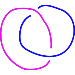
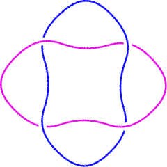
	L2a1 is [math]\displaystyle{ 2^2_1 }[/math] in Rolfsen's table of links. It is also known as the "Hopf Link". The sheet bend of practical knot tying deforms to the Hopf link when you tie the ends of each cord to itself.

Japanese family emblem	Linked hearts	expanded Kolam Two-hearts [1]	Logo
In Star of David form on old Jewish building in Prague	Three wreaths linked as two L2a1 configurations on Michelangelo's tomb	One form of a heterosexuality symbol	(pseudo-3D)
Are they forever linked? [2]	As impossible object	Linked hearts (pseudo-3D)	German coat of arms

Knot presentations

Planar diagram presentation	X4132 X2314
Gauss code	{1, -2}, {2, -1}

Polynomial invariants

Multivariable Alexander Polynomial (in [math]\displaystyle{ u }[/math], [math]\displaystyle{ v }[/math], [math]\displaystyle{ w }[/math], ...)	[math]\displaystyle{ -1 }[/math] (db)
Jones polynomial	[math]\displaystyle{ -\frac{1}{\sqrt{q}}-\frac{1}{q^{5/2}} }[/math] (db)
Signature	-1 (db)
HOMFLY-PT polynomial	[math]\displaystyle{ a^3 z^{-1} -z a-a z^{-1} }[/math] (db)
Kauffman polynomial	[math]\displaystyle{ -z a^3+a^3 z^{-1} -a^2-z a+a z^{-1} }[/math] (db)

Vassiliev invariants

V2 and V3:

(0, [math]\displaystyle{ -\frac{17}{48} }[/math])

V2,1 through V6,9:

V2,1 V3,1 V4,1 V4,2 V4,3 V5,1 V5,2 V5,3 V5,4 V6,1 V6,2 V6,3 V6,4 V6,5 V6,6 V6,7 V6,8 V6,9 Data:L2a1/V 2,1 Data:L2a1/V 3,1 Data:L2a1/V 4,1 Data:L2a1/V 4,2 Data:L2a1/V 4,3 Data:L2a1/V 5,1 Data:L2a1/V 5,2 Data:L2a1/V 5,3 Data:L2a1/V 5,4 Data:L2a1/V 6,1 Data:L2a1/V 6,2 Data:L2a1/V 6,3 Data:L2a1/V 6,4 Data:L2a1/V 6,5 Data:L2a1/V 6,6 Data:L2a1/V 6,7 Data:L2a1/V 6,8 Data:L2a1/V 6,9

V_2,1 through V_6,9 were provided by Petr Dunin-Barkowski <barkovs@itep.ru>, Andrey Smirnov <asmirnov@itep.ru>, and Alexei Sleptsov <sleptsov@itep.ru> and uploaded on October 2010 by User:Drorbn. Note that they are normalized differently than V₂ and V₃.

Khovanov Homology

The coefficients of the monomials [math]\displaystyle{ t^rq^j }[/math] are shown, along with their alternating sums [math]\displaystyle{ \chi }[/math] (fixed [math]\displaystyle{ j }[/math], alternation over [math]\displaystyle{ r }[/math]). The squares with yellow highlighting are those on the "critical diagonals", where [math]\displaystyle{ j-2r=s+1 }[/math] or [math]\displaystyle{ j-2r=s-1 }[/math], where [math]\displaystyle{ s= }[/math]-1 is the signature of L2a1. Nonzero entries off the critical diagonals (if any exist) are highlighted in red.

\   r    \    j   \ -2 -1 0 χ 0     1 1 -2     1 1 -4 1     1 -6 1     1

Integral Khovanov Homology (db, data source)

[math]\displaystyle{ \dim{\mathcal G}_{2r+i}\operatorname{KH}^r_{\mathbb Z} }[/math] [math]\displaystyle{ i=-2 }[/math] [math]\displaystyle{ i=0 }[/math] [math]\displaystyle{ r=-2 }[/math] [math]\displaystyle{ {\mathbb Z} }[/math] [math]\displaystyle{ {\mathbb Z} }[/math] [math]\displaystyle{ r=-1 }[/math] [math]\displaystyle{ r=0 }[/math] [math]\displaystyle{ {\mathbb Z} }[/math] [math]\displaystyle{ {\mathbb Z} }[/math]

Computer Talk

Much of the above data can be recomputed by Mathematica using the package KnotTheory`. See A Sample KnotTheory` Session.

[math]\displaystyle{ \textrm{Include}(\textrm{ColouredJonesM.mhtml}) }[/math]

In[1]:=	<< KnotTheory`
Loading KnotTheory` (version of August 17, 2005, 14:44:34)...
In[2]:=	Crossings[Link[2, Alternating, 1]]
Out[2]=	2
In[3]:=	PD[Link[2, Alternating, 1]]
Out[3]=	PD[X[4, 1, 3, 2], X[2, 3, 1, 4]]
In[4]:=	GaussCode[Link[2, Alternating, 1]]
Out[4]=	GaussCode[{1, -2}, {2, -1}]
In[5]:=	BR[Link[2, Alternating, 1]]
Out[5]=	BR[Link[2, Alternating, 1]]
In[6]:=	alex = Alexander[Link[2, Alternating, 1]][t]
Out[6]=	ComplexInfinity
In[7]:=	Conway[Link[2, Alternating, 1]][z]
Out[7]=	ComplexInfinity
In[8]:=	Select[AllKnots[], (alex === Alexander[#][t])&]
Out[8]=	{}
In[9]:=	{KnotDet[Link[2, Alternating, 1]], KnotSignature[Link[2, Alternating, 1]]}
Out[9]=	{Infinity, -1}
In[10]:=	J=Jones[Link[2, Alternating, 1]][q]
Out[10]=	-(5/2) 1 -q - ------- Sqrt[q]
In[11]:=	Select[AllKnots[], (J === Jones[#][q] || (J /. q-> 1/q) === Jones[#][q])&]
Out[11]=	{}
In[12]:=	A2Invariant[Link[2, Alternating, 1]][q]
Out[12]=	-10 2 2 2 -2 1 + q + -- + -- + -- + q 8 6 4 q q q
In[13]:=	Kauffman[Link[2, Alternating, 1]][a, z]
Out[13]=	3 2 a a 3 -a + - + -- - a z - a z z z
In[14]:=	{Vassiliev[2][Link[2, Alternating, 1]], Vassiliev[3][Link[2, Alternating, 1]]}
Out[14]=	17 {0, -(--)} 48
In[15]:=	Kh[Link[2, Alternating, 1]][q, t]
Out[15]=	-2 1 1 1 + q + ----- + ----- 6 2 4 2 q t q t