"Rubberband" Brunnian Links
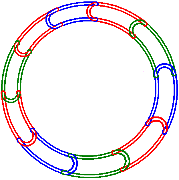
A "Rubberband" Brunnian link is obtained by connecting unknots in a closed chain as illustrated in the diagram of the 10-component link, where the last knot gets connected to the first one.
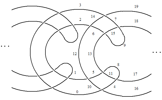
If we number the strands in one section of the link as shown and proceed with numbering each following section in the same manner, we can get its PD form. The PD of any "Rubberband" link can be generated in this way by varying the desired number of components:
(For In[1] see Setup)
In[2]:=
|
K0 =
  PD[X[1, 10, 5, 12], X[2, 12, 6, 14], X[5, 11, 8, 13],
   X[6, 13, 9, 15], X[10, 0, 16, 4], X[11, 4, 17, 8], X[14, 7, 19, 3],
    X[15, 9, 18, 7]];
|
In[3]:=
|
RubberBandBrunnian[n_] :=
 Join @@ Table[K0 /. j_Integer :> j + 16 k, {k, 0, n - 1}] /. {16
     n -> 0, 16 n + 1 -> 1, 16 n + 2 -> 2, 16 n + 3 -> 3}
|
For instance, let us draw the links with three, four, and five components and compute their Jones polynomials:
In[4]:=
|
RBB3=RubberBandBrunnian[3];
RBB4=RubberBandBrunnian[4];
RBB5=RubberBandBrunnian[5];
|
In[5]:=
|
DrawMorseLink/@{RBB3,RBB4,RBB5}
|
Out[5]=
|
{-Graphics-, -Graphics-, -Graphics-}
|
In[6]:=
|
RBJones= Jones[#][q] & /@ {RBB3, RBB4, RBB5}
|
Out[6]=
|
         2       3       4       5       7       8       9       10
{-q + 5 q  - 11 q  + 14 q  - 10 q  + 11 q  - 18 q  + 24 q  - 18 q   +

       11       13       14       15      16    17
   11 q   - 10 q   + 14 q   - 11 q   + 5 q   - q  ,

    3/2      5/2       7/2       9/2       11/2       13/2       15/2
  -q    + 7 q    - 24 q    + 49 q    - 56 q     + 18 q     + 51 q     -

        17/2        19/2        21/2       23/2       25/2
   111 q     + 131 q     - 100 q     + 32 q     + 32 q     -

        27/2        29/2        31/2       33/2       35/2       37/2
   100 q     + 131 q     - 111 q     + 51 q     + 18 q     - 56 q     +

       39/2       41/2      43/2    45/2
   49 q     - 24 q     + 7 q     - q    ,

    2      3       4        5        6        7       8        9
  -q  + 9 q  - 40 q  + 110 q  - 189 q  + 167 q  + 57 q  - 414 q  +

        10        11        12        13        14        15
   660 q   - 581 q   + 189 q   + 305 q   - 672 q   + 816 q   -

        16        17        18        19        20        21       22
   672 q   + 305 q   + 189 q   - 581 q   + 660 q   - 414 q   + 57 q   +

        23        24        25       26      27    28
   167 q   - 189 q   + 110 q   - 40 q   + 9 q   - q  }
|
We can also check that when one component is removed the remaining link is trivial:
In[7]:=
|
S = SubLink[RubberBandBrunnian[5], {1, 2, 3, 4}];
|
In[8]:=
|
J=Factor[Jones[S][q]]
|
Out[8]=
|
   6        3
-(q  (1 + q) )
|
Brunnian Braids
Similarly, in the case of Brunnian braids, removing one strand gives us a trivial braid. We can verify that using the following two programs. The first one constructs a Brunnian braid while the second one removes a selected strand:
In[9]:=
|
BR /: Inverse[BR[n_, l_List]] := BR[n, -Reverse[l]];
BR /: BR[n1_, l1_] ** BR[n2_, l2_] := BR[Max[n1, n2], Join[l1, l2]];
BrunnianBraid[2] = BR[2, {1, 1}];
BrunnianBraid[n_] /; n > 2 := Module[
  {b0},
  b0 = BrunnianBraid[n - 1];
  ((b0 ** BR[n, {n - 1, n - 1}]) ** Inverse[b0]) **
   BR[n, {1 - n, 1 - n}]
  ]
|
In[10]:=
|
DeleteStrand[k_, BR[n_, l_List]] := BR[n - 1, DeleteStrand[k, l]];
DeleteStrand[k_, {}] = {};
DeleteStrand[k_, {j1_, js___}] := Which[
  k < Abs[j1], {j1 - Sign[j1]}~Join~DeleteStrand[k, {js}],
  k == Abs[j1], DeleteStrand[k + 1, {js}],
  k == Abs[j1] + 1, DeleteStrand[k - 1, {js}],
  k > Abs[j1] + 1, {j1}~Join~DeleteStrand[k, {js}]
  ]
|
Testing for the Brunnian braid with four strands, we get:
In[12]:=
|
Jones[b][q]
|
Out[12]=
|
  -(11/2)    4      6      5      5        1                   3/2
-q        + ---- - ---- + ---- - ---- - ------- - Sqrt[q] - 5 q    +
             9/2    7/2    5/2    3/2   Sqrt[q]
            q      q      q      q

     5/2      7/2      9/2    11/2
  5 q    - 6 q    + 4 q    - q
|
In[14]:=
|
Jones[#][q] & /@ {bb, BR[3, {}]}
|
Out[14]=
|
     1          1
{2 + - + q, 2 + - + q}
     q          q
|

