Naming and Enumeration

KnotTheory`/Navigation  The Mathematica Package KnotTheory` Acknowledgement Setup Naming and Enumeration Presentations Planar Diagrams Some further details Gauss Codes DT (Dowker-Thistlethwaite) Codes Braid Representatives MorseLink Presentations Arc Presentations Conway Notation Graphical Input Graphical Output Drawing Planar Diagrams How does it work? Drawing MorseLink Presentations Drawing Braids Structure and Operations Invariants Invariants from Braid Theory Three Dimensional Invariants The Alexander-Conway Polynomial The Multivariable Alexander Polynomial The Determinant and the Signature The Jones Polynomial How is the Jones polynomial computed? The Coloured Jones Polynomials The A2 Invariant Quantum knot invariants The HOMFLY-PT Polynomial The Kauffman Polynomial Finite Type (Vassiliev) Invariants Khovanov Homology Heegaard Floer Knot Homology R-Matrix Invariants Extras Included with KnotTheory` Drawing with TubePlot Standalone_TubePlot Using the LinKnot package WikiLink QuantumGroups` Lightly Documented Features A Sample KnotTheory` Session Further Usage Example Prime Links with a Non-Prime Component "Rubberband" Brunnian Links Identifying Knots within a List Cabling Burau's Theorem Further Knot Theory Software KnotPlot Knotscape Xknots Extending/Modifying KnotTheory` Bugs How to Edit this Manual...

KnotTheory` comes loaded with some knot tables; currently, the Rolfsen table of prime knots with up to 10 crossings [Rolfsen], the Hoste-Thistlethwaite tables of prime knots with up to 16 crossings and the Thistlethwaite table of prime links with up to 11 crossings (see Knotscape):

(For In[1] see Setup)

In[1]:= ?Knot Knot[n, k] denotes the kth knot with n crossings in the Rolfsen table. Knot[11, Alternating, k] denotes the kth alternating 11-crossing knot in the Hoste-Thistlethwaite table. Knot[11, NonAlternating, k] denotes the kth non alternating 11-crossing knot in the Hoste-Thistlethwaite table.

In[2]:= ?Link Link[n, Alternating, k] denotes the kth alternating n-crossing link in the Thistlethwaite table. Link[n, NonAlternating, k] denotes the kth non alternating n-crossing link in the Thistlethwaite table.

6_1

9_46

Thus, for example, let us verify that the knots 6_1 and 9_46 have the same Alexander polynomial:

In[3]:=	Alexander[Knot[6, 1]][t]
Out[3]=	2 5 - - - 2 t t

In[4]:=	Alexander[Knot[9, 46]][t]
Out[4]=	2 5 - - - 2 t t

L6a4

We can also check that the Borromean rings, L6a4 in the Thistlethwaite table, is a 3-component link:

In[5]:=	Length[Skeleton[Link[6, Alternating, 4]]]
Out[5]=	3

In[6]:= ?AllKnots AllKnots[] return a list of all the named knots known to KnotTheory.m.

In[7]:= ?AllLinks AllLinks[] return a list of all the named links known to KnotTheory.m.

Thus at the moment there are 802 knots and 1424 links known to KnotTheory`:

In[8]:=	Length /@ {AllKnots[], AllLinks[]}
Out[8]=	{802, 1424}

In[10]:=	Show[DrawPD[Knot[13, NonAlternating, 5016], {Gap -> 0.025}]]
Out[10]=	-Graphics-

(Shumakovitch had noticed that this nice knot has interesting Khovanov homology; see [Shumakovitch]).

In addition to the tables, KnotTheory` also knows about torus knots:

In[11]:= ?TorusKnot TorusKnot[m, n] represents the (m,n) torus knot.

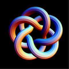T(5,3)

For example, the torus knots T(5,3) and T(3,5) have different presentations with different numbers of crossings, but they are in fact isotopic, and hence they have the same invariants (and in particular the same type 3 Vassiliev invariant $V_{3}$):

In[12]:=	Crossings /@ {TorusKnot[5,3], TorusKnot[3, 5]}
Out[12]=	{10, 12}

In[13]:=	Vassiliev[3] /@ {TorusKnot[5,3], TorusKnot[3, 5]}
Out[13]=	{20, 20}

KnotTheory` knows how to plot torus knots; see Drawing with TubePlot.

References

[Rolfsen] ^  D. Rolfsen, Knots and Links, Publish or Perish, Mathematics Lecture Series 7, Wilmington 1976.

[Shumakovitch] ^  A. Shumakovitch, Torsion of the Khovanov Homology, arXiv:math.GT/0405474.