8 17: Difference between revisions
No edit summary |
DrorsRobot (talk | contribs) No edit summary |
||
| Line 1: | Line 1: | ||
<!-- WARNING! WARNING! WARNING! |
|||
<!-- This page was |
<!-- This page was generated from the splice template [[Rolfsen_Splice_Base]]. Please do not edit! |
||
<!-- --> <!-- |
|||
<!-- You probably want to edit the template referred to immediately below. (See [[Category:Knot Page Template]].) |
|||
--> |
|||
<!-- This page itself was created by running [[Media:KnotPageSpliceRobot.nb]] on [[Rolfsen_Splice_Base]]. --> |
|||
<!-- <math>\text{Null}</math> --> |
|||
<!-- <math>\text{Null}</math> --> |
|||
{{Rolfsen Knot Page| |
{{Rolfsen Knot Page| |
||
n = 8 | |
n = 8 | |
||
| Line 47: | Line 50: | ||
<td align=left><pre style="color: red; border: 0px; padding: 0em"><< KnotTheory`</pre></td> |
<td align=left><pre style="color: red; border: 0px; padding: 0em"><< KnotTheory`</pre></td> |
||
</tr> |
</tr> |
||
<tr valign=top><td colspan=2>Loading KnotTheory` (version of August 29, 2005, 15: |
<tr valign=top><td colspan=2>Loading KnotTheory` (version of August 29, 2005, 15:27:48)...</td></tr> |
||
<tr valign=top><td><pre style="color: blue; border: 0px; padding: 0em"><nowiki>In[2]:=</nowiki></pre></td><td><pre style="color: red; border: 0px; padding: 0em"><nowiki>PD[Knot[8, 17]]</nowiki></pre></td></tr> |
<tr valign=top><td><pre style="color: blue; border: 0px; padding: 0em"><nowiki>In[2]:=</nowiki></pre></td><td><pre style="color: red; border: 0px; padding: 0em"><nowiki>PD[Knot[8, 17]]</nowiki></pre></td></tr> |
||
<tr valign=top><td><pre style="color: blue; border: 0px; padding: 0em"><nowiki>Out[2]= </nowiki></pre></td><td><pre style="color: black; border: 0px; padding: 0em"><nowiki>PD[X[6, 2, 7, 1], X[14, 8, 15, 7], X[8, 3, 9, 4], X[2, 13, 3, 14], |
<tr valign=top><td><pre style="color: blue; border: 0px; padding: 0em"><nowiki>Out[2]= </nowiki></pre></td><td><pre style="color: black; border: 0px; padding: 0em"><nowiki>PD[X[6, 2, 7, 1], X[14, 8, 15, 7], X[8, 3, 9, 4], X[2, 13, 3, 14], |
||
| Line 63: | Line 66: | ||
<tr valign=top><td><pre style="color: blue; border: 0px; padding: 0em"><nowiki>Out[7]= </nowiki></pre></td><td><pre style="color: black; border: 0px; padding: 0em"><nowiki>3</nowiki></pre></td></tr> |
<tr valign=top><td><pre style="color: blue; border: 0px; padding: 0em"><nowiki>Out[7]= </nowiki></pre></td><td><pre style="color: black; border: 0px; padding: 0em"><nowiki>3</nowiki></pre></td></tr> |
||
<tr valign=top><td><pre style="color: blue; border: 0px; padding: 0em"><nowiki>In[8]:=</nowiki></pre></td><td><pre style="color: red; border: 0px; padding: 0em"><nowiki>Show[DrawMorseLink[Knot[8, 17]]]</nowiki></pre></td></tr><tr><td></td><td align=left>[[Image:8_17_ML.gif]]</td></tr><tr valign=top><td><tt><font color=blue>Out[8]=</font></tt><td><tt><font color=black>-Graphics-</font></tt></td></tr> |
<tr valign=top><td><pre style="color: blue; border: 0px; padding: 0em"><nowiki>In[8]:=</nowiki></pre></td><td><pre style="color: red; border: 0px; padding: 0em"><nowiki>Show[DrawMorseLink[Knot[8, 17]]]</nowiki></pre></td></tr><tr><td></td><td align=left>[[Image:8_17_ML.gif]]</td></tr><tr valign=top><td><tt><font color=blue>Out[8]=</font></tt><td><tt><font color=black>-Graphics-</font></tt></td></tr> |
||
<tr valign=top><td><pre style="color: blue; border: 0px; padding: 0em"><nowiki>In[9]:=</nowiki></pre></td><td><pre style="color: red; border: 0px; padding: 0em"><nowiki>(#[Knot[8, 17]]&) /@ { |
<tr valign=top><td><pre style="color: blue; border: 0px; padding: 0em"><nowiki>In[9]:=</nowiki></pre></td><td><pre style="color: red; border: 0px; padding: 0em"><nowiki> (#[Knot[8, 17]]&) /@ { |
||
SymmetryType, UnknottingNumber, ThreeGenus, |
|||
BridgeIndex, SuperBridgeIndex, NakanishiIndex |
|||
}</nowiki></pre></td></tr> |
|||
<tr valign=top><td><pre style="color: blue; border: 0px; padding: 0em"><nowiki>Out[9]= </nowiki></pre></td><td><pre style="color: black; border: 0px; padding: 0em"><nowiki>{NegativeAmphicheiral, 1, 3, 3, 4, 1}</nowiki></pre></td></tr> |
<tr valign=top><td><pre style="color: blue; border: 0px; padding: 0em"><nowiki>Out[9]= </nowiki></pre></td><td><pre style="color: black; border: 0px; padding: 0em"><nowiki>{NegativeAmphicheiral, 1, 3, 3, 4, 1}</nowiki></pre></td></tr> |
||
<tr valign=top><td><pre style="color: blue; border: 0px; padding: 0em"><nowiki>In[10]:=</nowiki></pre></td><td><pre style="color: red; border: 0px; padding: 0em"><nowiki>alex = Alexander[Knot[8, 17]][t]</nowiki></pre></td></tr> |
<tr valign=top><td><pre style="color: blue; border: 0px; padding: 0em"><nowiki>In[10]:=</nowiki></pre></td><td><pre style="color: red; border: 0px; padding: 0em"><nowiki>alex = Alexander[Knot[8, 17]][t]</nowiki></pre></td></tr> |
||
Revision as of 17:47, 31 August 2005
|
|
|
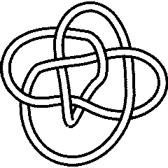 (KnotPlot image) |
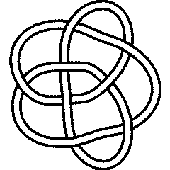
See the full Rolfsen Knot Table. Visit 8 17's page at the Knot Server (KnotPlot driven, includes 3D interactive images!) |
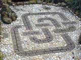 A knot in Brian Sanderson's Garden [1] |
Knot presentations
| Planar diagram presentation | X6271 X14,8,15,7 X8394 X2,13,3,14 X12,5,13,6 X4,9,5,10 X16,12,1,11 X10,16,11,15 |
| Gauss code | 1, -4, 3, -6, 5, -1, 2, -3, 6, -8, 7, -5, 4, -2, 8, -7 |
| Dowker-Thistlethwaite code | 6 8 12 14 4 16 2 10 |
| Conway Notation | [.2.2] |
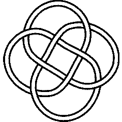
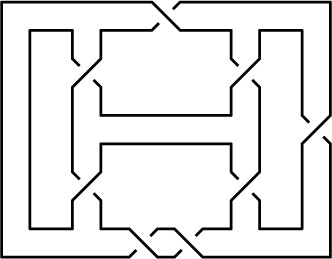
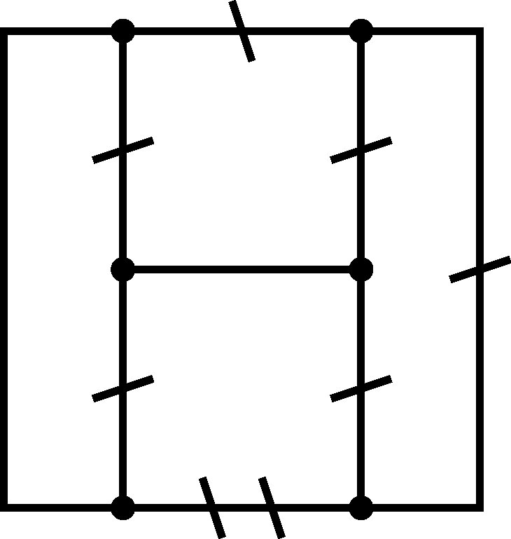
| Minimum Braid Representative | A Morse Link Presentation | An Arc Presentation | |||
Length is 8, width is 3, Braid index is 3 |
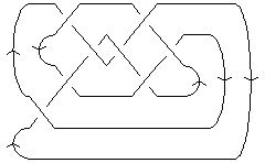
|
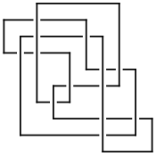 [{7, 10}, {9, 2}, {10, 4}, {3, 5}, {4, 8}, {6, 9}, {5, 1}, {2, 7}, {1, 6}, {8, 3}] |
[edit Notes on presentations of 8 17]
KnotTheory`. Your input (in red) is realistic; all else should have the same content as in a real mathematica session, but with different formatting.
(The path below may be different on your system, and possibly also the KnotTheory` date)
In[1]:=
|
AppendTo[$Path, "C:/drorbn/projects/KAtlas/"];
<< KnotTheory`
|
Loading KnotTheory` version of May 31, 2006, 14:15:20.091.
|
In[3]:=
|
K = Knot["8 17"];
|
In[4]:=
|
PD[K]
|
KnotTheory::loading: Loading precomputed data in PD4Knots`.
|
Out[4]=
|
X6271 X14,8,15,7 X8394 X2,13,3,14 X12,5,13,6 X4,9,5,10 X16,12,1,11 X10,16,11,15 |
In[5]:=
|
GaussCode[K]
|
Out[5]=
|
1, -4, 3, -6, 5, -1, 2, -3, 6, -8, 7, -5, 4, -2, 8, -7 |
In[6]:=
|
DTCode[K]
|
Out[6]=
|
6 8 12 14 4 16 2 10 |
(The path below may be different on your system)
In[7]:=
|
AppendTo[$Path, "C:/bin/LinKnot/"];
|
In[8]:=
|
ConwayNotation[K]
|
Out[8]=
|
[.2.2] |
In[9]:=
|
br = BR[K]
|
KnotTheory::credits: The minimum braids representing the knots with up to 10 crossings were provided by Thomas Gittings. See arXiv:math.GT/0401051.
|
Out[9]=
|
In[10]:=
|
{First[br], Crossings[br], BraidIndex[K]}
|
KnotTheory::credits: The braid index data known to KnotTheory` is taken from Charles Livingston's http://www.indiana.edu/~knotinfo/.
|
KnotTheory::loading: Loading precomputed data in IndianaData`.
|
Out[10]=
|
{ 3, 8, 3 } |
In[11]:=
|
Show[BraidPlot[br]]
|
Out[11]=
|
-Graphics- |
In[12]:=
|
Show[DrawMorseLink[K]]
|
KnotTheory::credits: "MorseLink was added to KnotTheory` by Siddarth Sankaran at the University of Toronto in the summer of 2005."
|
KnotTheory::credits: "DrawMorseLink was written by Siddarth Sankaran at the University of Toronto in the summer of 2005."
|

|
Out[12]=
|
-Graphics- |
In[13]:=
|
ap = ArcPresentation[K]
|
Out[13]=
|
ArcPresentation[{7, 10}, {9, 2}, {10, 4}, {3, 5}, {4, 8}, {6, 9}, {5, 1}, {2, 7}, {1, 6}, {8, 3}] |
In[14]:=
|
Draw[ap]
|

|
Out[14]=
|
-Graphics- |
Three dimensional invariants
|
[edit Notes for 8 17's three dimensional invariants] 8_17 is the first negatively amphicheiral knot in the Rolfsen Table. Namely, it is equal to the inverse of its mirror, yet it is different from both its inverse and its mirror. |
Four dimensional invariants
|
Polynomial invariants
A1 Invariants.
| Weight | Invariant |
|---|---|
| 1 | |
| 2 | |
| 3 | |
| 4 | |
| 5 | |
| 6 |
A2 Invariants.
| Weight | Invariant |
|---|---|
| 1,0 | |
| 1,1 | |
| 2,0 |
A3 Invariants.
| Weight | Invariant |
|---|---|
| 0,1,0 | |
| 1,0,0 | |
| 1,0,1 |
A4 Invariants.
| Weight | Invariant |
|---|---|
| 0,1,0,0 | |
| 1,0,0,0 |
B2 Invariants.
| Weight | Invariant |
|---|---|
| 0,1 | |
| 1,0 |
D4 Invariants.
| Weight | Invariant |
|---|---|
| 1,0,0,0 |
G2 Invariants.
| Weight | Invariant |
|---|---|
| 1,0 |
.
KnotTheory`, as shown in the (simulated) Mathematica session below. Your input (in red) is realistic; all else should have the same content as in a real mathematica session, but with different formatting. This Mathematica session is also available (albeit only for the knot 5_2) as the notebook PolynomialInvariantsSession.nb.
(The path below may be different on your system, and possibly also the KnotTheory` date)
In[1]:=
|
AppendTo[$Path, "C:/drorbn/projects/KAtlas/"];
<< KnotTheory`
|
Loading KnotTheory` version of August 31, 2006, 11:25:27.5625.
|
In[3]:=
|
K = Knot["8 17"];
|
In[4]:=
|
Alexander[K][t]
|
KnotTheory::loading: Loading precomputed data in PD4Knots`.
|
Out[4]=
|
In[5]:=
|
Conway[K][z]
|
Out[5]=
|
In[6]:=
|
Alexander[K, 2][t]
|
KnotTheory::credits: The program Alexander[K, r] to compute Alexander ideals was written by Jana Archibald at the University of Toronto in the summer of 2005.
|
Out[6]=
|
In[7]:=
|
{KnotDet[K], KnotSignature[K]}
|
Out[7]=
|
{ 37, 0 } |
In[8]:=
|
Jones[K][q]
|
KnotTheory::loading: Loading precomputed data in Jones4Knots`.
|
Out[8]=
|
In[9]:=
|
HOMFLYPT[K][a, z]
|
KnotTheory::credits: The HOMFLYPT program was written by Scott Morrison.
|
Out[9]=
|
In[10]:=
|
Kauffman[K][a, z]
|
KnotTheory::loading: Loading precomputed data in Kauffman4Knots`.
|
Out[10]=
|
"Similar" Knots (within the Atlas)
Same Alexander/Conway Polynomial: {K11n53,}
Same Jones Polynomial (up to mirroring, ): {}
KnotTheory`. Your input (in red) is realistic; all else should have the same content as in a real mathematica session, but with different formatting.
(The path below may be different on your system, and possibly also the KnotTheory` date)
In[1]:=
|
AppendTo[$Path, "C:/drorbn/projects/KAtlas/"];
<< KnotTheory`
|
Loading KnotTheory` version of May 31, 2006, 14:15:20.091.
|
In[3]:=
|
K = Knot["8 17"];
|
In[4]:=
|
{A = Alexander[K][t], J = Jones[K][q]}
|
KnotTheory::loading: Loading precomputed data in PD4Knots`.
|
KnotTheory::loading: Loading precomputed data in Jones4Knots`.
|
Out[4]=
|
{ , } |
In[5]:=
|
DeleteCases[Select[AllKnots[], (A === Alexander[#][t]) &], K]
|
KnotTheory::loading: Loading precomputed data in DTCode4KnotsTo11`.
|
KnotTheory::credits: The GaussCode to PD conversion was written by Siddarth Sankaran at the University of Toronto in the summer of 2005.
|
Out[5]=
|
{K11n53,} |
In[6]:=
|
DeleteCases[
  Select[
    AllKnots[],
    (J === Jones[#][q] || (J /. q -> 1/q) === Jones[#][q]) &
    ],
  K
  ]
|
KnotTheory::loading: Loading precomputed data in Jones4Knots11`.
|
Out[6]=
|
{} |
Vassiliev invariants
| V2 and V3: | (-1, 0) |
| V2,1 through V6,9: |
|
V2,1 through V6,9 were provided by Petr Dunin-Barkowski <barkovs@itep.ru>, Andrey Smirnov <asmirnov@itep.ru>, and Alexei Sleptsov <sleptsov@itep.ru> and uploaded on October 2010 by User:Drorbn. Note that they are normalized differently than V2 and V3.
Khovanov Homology
| The coefficients of the monomials are shown, along with their alternating sums (fixed , alternation over ). The squares with yellow highlighting are those on the "critical diagonals", where or , where 0 is the signature of 8 17. Nonzero entries off the critical diagonals (if any exist) are highlighted in red. |
|
| Integral Khovanov Homology
(db, data source) |
|
The Coloured Jones Polynomials
| 2 | |
| 3 | |
| 4 | |
| 5 | |
| 6 | |
| 7 |
Computer Talk
Much of the above data can be recomputed by Mathematica using the package KnotTheory`. See A Sample KnotTheory` Session, or any of the Computer Talk sections above.
Modifying This Page
| Read me first: Modifying Knot Pages
See/edit the Rolfsen Knot Page master template (intermediate). See/edit the Rolfsen_Splice_Base (expert). Back to the top. |
|
