Graphical Input: Difference between revisions
From Knot Atlas
Jump to navigationJump to search
No edit summary |
DrorsRobot (talk | contribs) No edit summary |
||
| (6 intermediate revisions by 3 users not shown) | |||
| Line 2: | Line 2: | ||
Thanks to our link with [[Using the LinKnot package|LinKnot]], on Windows systems <tt>KnotTheory`</tt> accepts graphical knot input. |
Thanks to our link with [[Using the LinKnot package|LinKnot]], on Windows systems <tt>KnotTheory`</tt> accepts graphical knot input. |
||
{{Startup Note}} |
{{Startup Note}} |
||
| Line 20: | Line 19: | ||
n = 3 | |
n = 3 | |
||
n1 = 4 | |
n1 = 4 | |
||
in = <nowiki> |
in = <nowiki>KnotInput</nowiki> | |
||
out= <nowiki>KnotInput[] opens a window in which you can draw a knot or link by hand. Right click and select 'Quit' when you're done. This function requires the package LinKnots`, and will only run on Windows machines. Sorry!</nowiki> | |
|||
out= <nowiki>ConwayNotation[s] represents the knot or link whose Conway notation is the string s. ConwayNotation[K], where K is a knot or a link with up to 12 crossings, returns ConwayNotation[s], where s is a string containing the Conway notation of K.</nowiki> | |
|||
about= <nowiki>The program |
about= <nowiki>The KnotInput program was written by M. Ochiai, C. Nakai, Y. Matsuyama and N. Imafuji and is imported to KnotTheory` via the package LinKnot by S. Jablan and R. Sazdanovic</nowiki>}} |
||
<!--END--> |
|||
Thus for example, the input line |
|||
{{In| |
|||
n = 5 | |
|||
in = <nowiki>K = KnotInput[]</nowiki>}} |
|||
pops a blank window on which a knot or a link can be drawn with mouse clicks. At first pass all crossings are drawn as "new over old", but a further click on any given crossing will flip it. |
|||
[[Image:KnotInput_Screenshot.png|thumb|center|304px|<tt>KnotInput</tt> in action.]] |
|||
A right click followed by selecting "quit" will then determine the Gauss code of the knot or link just drawn and return it to Mathematica: |
|||
{{Out| |
|||
n = 5 | |
|||
out = <nowiki>GaussCode[{-1,-4,2,3},{-3,-5,4,6},{5,1,-6,-2}]</nowiki>}} |
|||
<tt>K</tt> is now perfectly usable within <tt>KnotTheory`</tt>: |
|||
<!--$K=GaussCode[{-1,-4,2,3},{-3,-5,4,6},{5,1,-6,-2}];++n;$--><!--END--> |
|||
<!--$$Kh[K][q, t]$$--> |
|||
<!--Robot Land, no human edits to "END"--> |
|||
{{InOut| |
|||
n = 5 | |
|||
in = <nowiki>Kh[K][q, t]</nowiki> | |
|||
out= <nowiki> 3 5 7 2 11 3 9 4 11 4 13 4 |
|||
q + q + q t + q t + q t + 3 q t + 2 q t</nowiki>}} |
|||
<!--END--> |
<!--END--> |
||
Latest revision as of 20:33, 31 March 2006
Thanks to our link with LinKnot, on Windows systems KnotTheory` accepts graphical knot input.
(For In[1] see Setup)
As in the section Using the LinKnot package, the first step is to add LinKnot to the Mathematica search path. This path will likely be different on your computer.
In[2]:=
|
AppendTo[$Path, "C:/bin/LinKnot/"];
|
|
| ||||||||
Thus for example, the input line
In[5]:=
|
K = KnotInput[]
|
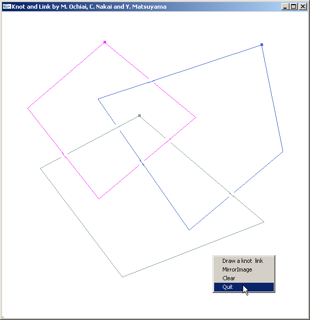
pops a blank window on which a knot or a link can be drawn with mouse clicks. At first pass all crossings are drawn as "new over old", but a further click on any given crossing will flip it.
A right click followed by selecting "quit" will then determine the Gauss code of the knot or link just drawn and return it to Mathematica:
Out[5]=
|
GaussCode[{-1,-4,2,3},{-3,-5,4,6},{5,1,-6,-2}]
|
K is now perfectly usable within KnotTheory`:
In[5]:=
|
Kh[K][q, t]
|
Out[5]=
|
 3    5    7  2    11  3    9  4      11  4      13  4
q  + q  + q  t  + q   t  + q  t  + 3 q   t  + 2 q   t
|
