9_42 is Alexander Stoimenow's favourite knot!
 Alsacian chair, alsacian museum, Strasbourg, France |
|
Knot presentations
| Planar diagram presentation
|
X1425 X5,10,6,11 X3948 X9,3,10,2 X16,12,17,11 X14,7,15,8 X6,15,7,16 X18,14,1,13 X12,18,13,17
|
| Gauss code
|
-1, 4, -3, 1, -2, -7, 6, 3, -4, 2, 5, -9, 8, -6, 7, -5, 9, -8
|
| Dowker-Thistlethwaite code
|
4 8 10 -14 2 -16 -18 -6 -12
|
| Conway Notation
|
[22,3,2-]
|
| Minimum Braid Representative
|
A Morse Link Presentation
|
An Arc Presentation
|
Length is 9, width is 4,
Braid index is 4
|
|
[{11, 2}, {1, 9}, {10, 5}, {9, 11}, {8, 4}, {2, 7}, {6, 8}, {7, 10}, {5, 3}, {4, 1}, {3, 6}]
|
[edit Notes on presentations of 9 42]
|
|
|
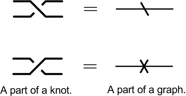 A part of a knot and a part of a graph. |
Computer Talk
The above data is available with the
Mathematica package
KnotTheory`. Your input (in
red) is realistic; all else should have the same content as in a real mathematica session, but with different formatting.
(The path below may be different on your system, and possibly also the KnotTheory` date)
In[1]:=
|
AppendTo[$Path, "C:/drorbn/projects/KAtlas/"];
<< KnotTheory`
|
In[3]:=
|
K = Knot["9 42"];
|
|
|
KnotTheory::loading: Loading precomputed data in PD4Knots`.
|
Out[4]=
|
X1425 X5,10,6,11 X3948 X9,3,10,2 X16,12,17,11 X14,7,15,8 X6,15,7,16 X18,14,1,13 X12,18,13,17
|
Out[5]=
|
-1, 4, -3, 1, -2, -7, 6, 3, -4, 2, 5, -9, 8, -6, 7, -5, 9, -8
|
Out[6]=
|
4 8 10 -14 2 -16 -18 -6 -12
|
(The path below may be different on your system)
In[7]:=
|
AppendTo[$Path, "C:/bin/LinKnot/"];
|
In[8]:=
|
ConwayNotation[K]
|
|
|
KnotTheory::credits: The minimum braids representing the knots with up to 10 crossings were provided by Thomas Gittings. See arXiv:math.GT/0401051.
|
Out[9]=
|

|
In[10]:=
|
{First[br], Crossings[br], BraidIndex[K]}
|
|
|
KnotTheory::loading: Loading precomputed data in IndianaData`.
|
In[11]:=
|
Show[BraidPlot[br]]
|
In[12]:=
|
Show[DrawMorseLink[K]]
|
|
|
KnotTheory::credits: "MorseLink was added to KnotTheory` by Siddarth Sankaran at the University of Toronto in the summer of 2005."
|
|
|
KnotTheory::credits: "DrawMorseLink was written by Siddarth Sankaran at the University of Toronto in the summer of 2005."
|
In[13]:=
|
ap = ArcPresentation[K]
|
Out[13]=
|
ArcPresentation[{11, 2}, {1, 9}, {10, 5}, {9, 11}, {8, 4}, {2, 7}, {6, 8}, {7, 10}, {5, 3}, {4, 1}, {3, 6}]
|
Four dimensional invariants
Polynomial invariants
| Alexander polynomial |
 |
| Conway polynomial |
 |
| 2nd Alexander ideal (db, data sources) |
 |
| Determinant and Signature |
{ 7, 2 } |
| Jones polynomial |
 |
| HOMFLY-PT polynomial (db, data sources) |
 |
| Kauffman polynomial (db, data sources) |
 |
| The A2 invariant |
 |
| The G2 invariant |
 |
Further Quantum Invariants
Further quantum knot invariants for 9_42.
A1 Invariants.
| Weight
|
Invariant
|
| 1
|

|
| 2
|

|
| 3
|

|
| 4
|

|
| 5
|

|
A2 Invariants.
| Weight
|
Invariant
|
| 1,0
|
|
| 1,1
|

|
| 2,0
|

|
A3 Invariants.
| Weight
|
Invariant
|
| 0,1,0
|

|
| 1,0,0
|

|
A4 Invariants.
| Weight
|
Invariant
|
| 0,1,0,0
|

|
| 1,0,0,0
|

|
B2 Invariants.
| Weight
|
Invariant
|
| 0,1
|

|
| 1,0
|

|
D4 Invariants.
| Weight
|
Invariant
|
| 1,0,0,0
|

|
G2 Invariants.
| Weight
|
Invariant
|
| 1,0
|
|
.
Computer Talk
The above data is available with the
Mathematica package
KnotTheory`, as shown in the (simulated) Mathematica session below. Your input (in
red) is realistic; all else should have the same content as in a real mathematica session, but with different formatting. This Mathematica session is also available (albeit only for the knot
5_2) as the notebook
PolynomialInvariantsSession.nb.
(The path below may be different on your system, and possibly also the KnotTheory` date)
In[1]:=
|
AppendTo[$Path, "C:/drorbn/projects/KAtlas/"];
<< KnotTheory`
|
In[3]:=
|
K = Knot["9 42"];
|
|
|
KnotTheory::loading: Loading precomputed data in PD4Knots`.
|
Out[4]=
|
|
Out[5]=
|
|
In[6]:=
|
Alexander[K, 2][t]
|
|
|
KnotTheory::credits: The program Alexander[K, r] to compute Alexander ideals was written by Jana Archibald at the University of Toronto in the summer of 2005.
|
Out[6]=
|
|
In[7]:=
|
{KnotDet[K], KnotSignature[K]}
|
|
|
KnotTheory::loading: Loading precomputed data in Jones4Knots`.
|
Out[8]=
|
|
In[9]:=
|
HOMFLYPT[K][a, z]
|
|
|
KnotTheory::credits: The HOMFLYPT program was written by Scott Morrison.
|
Out[9]=
|
|
In[10]:=
|
Kauffman[K][a, z]
|
|
|
KnotTheory::loading: Loading precomputed data in Kauffman4Knots`.
|
Out[10]=
|
|
"Similar" Knots (within the Atlas)
Same Alexander/Conway Polynomial:
{}
Same Jones Polynomial (up to mirroring,  ):
{}
):
{}
Computer Talk
The above data is available with the
Mathematica package
KnotTheory`. Your input (in
red) is realistic; all else should have the same content as in a real mathematica session, but with different formatting.
(The path below may be different on your system, and possibly also the KnotTheory` date)
In[1]:=
|
AppendTo[$Path, "C:/drorbn/projects/KAtlas/"];
<< KnotTheory`
|
In[3]:=
|
K = Knot["9 42"];
|
In[4]:=
|
{A = Alexander[K][t], J = Jones[K][q]}
|
|
|
KnotTheory::loading: Loading precomputed data in PD4Knots`.
|
|
|
KnotTheory::loading: Loading precomputed data in Jones4Knots`.
|
Out[4]=
|
{ , }
|
In[5]:=
|
DeleteCases[Select[AllKnots[], (A === Alexander[#][t]) &], K]
|
|
|
KnotTheory::loading: Loading precomputed data in DTCode4KnotsTo11`.
|
|
|
KnotTheory::credits: The GaussCode to PD conversion was written by Siddarth Sankaran at the University of Toronto in the summer of 2005.
|
In[6]:=
|
DeleteCases[
  Select[
    AllKnots[],
    (J === Jones[#][q] || (J /. q -> 1/q) === Jones[#][q]) &
    ],
  K
  ]
|
|
|
KnotTheory::loading: Loading precomputed data in Jones4Knots11`.
|
| V2,1 through V6,9:
|
| V2,1
|
V3,1
|
V4,1
|
V4,2
|
V4,3
|
V5,1
|
V5,2
|
V5,3
|
V5,4
|
V6,1
|
V6,2
|
V6,3
|
V6,4
|
V6,5
|
V6,6
|
V6,7
|
V6,8
|
V6,9
|

|

|

|

|

|
|
|
|
|

|
|

|

|

|

|

|

|

|
|
V2,1 through V6,9 were provided by Petr Dunin-Barkowski <barkovs@itep.ru>, Andrey Smirnov <asmirnov@itep.ru>, and Alexei Sleptsov <sleptsov@itep.ru> and uploaded on October 2010 by User:Drorbn. Note that they are normalized differently than V2 and V3.
The coefficients of the monomials  are shown, along with their alternating sums are shown, along with their alternating sums  (fixed (fixed  , alternation over , alternation over  ). The squares with yellow highlighting are those on the "critical diagonals", where ). The squares with yellow highlighting are those on the "critical diagonals", where  or or  , where , where  2 is the signature of 9 42. Nonzero entries off the critical diagonals (if any exist) are highlighted in red. 2 is the signature of 9 42. Nonzero entries off the critical diagonals (if any exist) are highlighted in red.
|
|
|
-4 | -3 | -2 | -1 | 0 | 1 | 2 | χ |
| 7 | | | | | | | 1 | 1 |
| 5 | | | | | | | | 0 |
| 3 | | | | | 1 | 1 | | 0 |
| 1 | | | | 1 | 1 | | | 0 |
| -1 | | | | 1 | 1 | | | 0 |
| -3 | | 1 | 1 | | | | | 0 |
| -5 | | | | | | | | 0 |
| -7 | 1 | | | | | | | 1 |
|
The Coloured Jones Polynomials