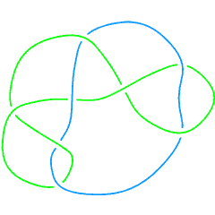
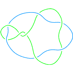
L8a10

L8a9

L8a11

	Visit L8a10's page at Knotilus! Visit L8a10's page at the original Knot Atlas!
	L8a10 is [math]\displaystyle{ 8^2_{5} }[/math] in the Rolfsen table of links.

Symmetric version

Mongolian ornament

Knot presentations

Planar diagram presentation	X8192 X10,3,11,4 X12,15,13,16 X14,5,15,6 X4,13,5,14 X16,11,7,12 X2738 X6,9,1,10
Gauss code	{1, -7, 2, -5, 4, -8}, {7, -1, 8, -2, 6, -3, 5, -4, 3, -6}

Polynomial invariants

Multivariable Alexander Polynomial (in [math]\displaystyle{ u }[/math], [math]\displaystyle{ v }[/math], [math]\displaystyle{ w }[/math], ...)	[math]\displaystyle{ -\frac{2 t(2) t(1)^2-t(1)^2+2 t(2)^2 t(1)-3 t(2) t(1)+2 t(1)-t(2)^2+2 t(2)}{t(1) t(2)} }[/math] (db)
Jones polynomial	[math]\displaystyle{ -\frac{1}{q^{3/2}}+\frac{2}{q^{5/2}}-\frac{4}{q^{7/2}}+\frac{4}{q^{9/2}}-\frac{5}{q^{11/2}}+\frac{4}{q^{13/2}}-\frac{3}{q^{15/2}}+\frac{2}{q^{17/2}}-\frac{1}{q^{19/2}} }[/math] (db)
Signature	-3 (db)
HOMFLY-PT polynomial	[math]\displaystyle{ a^9 z-a^7 z^3+a^7 z^{-1} -2 a^5 z^3-3 a^5 z-a^5 z^{-1} -a^3 z^3-a^3 z }[/math] (db)
Kauffman polynomial	[math]\displaystyle{ -z^5 a^{11}+3 z^3 a^{11}-2 z a^{11}-2 z^6 a^{10}+6 z^4 a^{10}-4 z^2 a^{10}-z^7 a^9+4 z^3 a^9-z a^9-4 z^6 a^8+8 z^4 a^8-3 z^2 a^8-z^7 a^7-2 z^5 a^7+6 z^3 a^7-4 z a^7+a^7 z^{-1} -2 z^6 a^6+2 z^2 a^6-a^6-3 z^5 a^5+4 z^3 a^5-4 z a^5+a^5 z^{-1} -2 z^4 a^4+z^2 a^4-z^3 a^3+z a^3 }[/math] (db)

Vassiliev invariants

V2 and V3:

(0, [math]\displaystyle{ -\frac{177}{16} }[/math])

V2,1 through V6,9:

V2,1 V3,1 V4,1 V4,2 V4,3 V5,1 V5,2 V5,3 V5,4 V6,1 V6,2 V6,3 V6,4 V6,5 V6,6 V6,7 V6,8 V6,9 Data:L8a10/V 2,1 Data:L8a10/V 3,1 Data:L8a10/V 4,1 Data:L8a10/V 4,2 Data:L8a10/V 4,3 Data:L8a10/V 5,1 Data:L8a10/V 5,2 Data:L8a10/V 5,3 Data:L8a10/V 5,4 Data:L8a10/V 6,1 Data:L8a10/V 6,2 Data:L8a10/V 6,3 Data:L8a10/V 6,4 Data:L8a10/V 6,5 Data:L8a10/V 6,6 Data:L8a10/V 6,7 Data:L8a10/V 6,8 Data:L8a10/V 6,9

V_2,1 through V_6,9 were provided by Petr Dunin-Barkowski <barkovs@itep.ru>, Andrey Smirnov <asmirnov@itep.ru>, and Alexei Sleptsov <sleptsov@itep.ru> and uploaded on October 2010 by User:Drorbn. Note that they are normalized differently than V₂ and V₃.

Khovanov Homology

The coefficients of the monomials [math]\displaystyle{ t^rq^j }[/math] are shown, along with their alternating sums [math]\displaystyle{ \chi }[/math] (fixed [math]\displaystyle{ j }[/math], alternation over [math]\displaystyle{ r }[/math]). The squares with yellow highlighting are those on the "critical diagonals", where [math]\displaystyle{ j-2r=s+1 }[/math] or [math]\displaystyle{ j-2r=s-1 }[/math], where [math]\displaystyle{ s= }[/math]-3 is the signature of L8a10. Nonzero entries off the critical diagonals (if any exist) are highlighted in red.

\   r    \    j   \ -8 -7 -6 -5 -4 -3 -2 -1 0 χ -2                 1 1 -4               2 1 -1 -6             2     2 -8           2 2     0 -10         3 2       1 -12       1 2         1 -14     2 3           -1 -16   1 2             1 -18   1               -1 -20 1                 1

Integral Khovanov Homology (db, data source)

[math]\displaystyle{ \dim{\mathcal G}_{2r+i}\operatorname{KH}^r_{\mathbb Z} }[/math] [math]\displaystyle{ i=-4 }[/math] [math]\displaystyle{ i=-2 }[/math] [math]\displaystyle{ r=-8 }[/math] [math]\displaystyle{ {\mathbb Z} }[/math] [math]\displaystyle{ r=-7 }[/math] [math]\displaystyle{ {\mathbb Z}\oplus{\mathbb Z}_2 }[/math] [math]\displaystyle{ {\mathbb Z} }[/math] [math]\displaystyle{ r=-6 }[/math] [math]\displaystyle{ {\mathbb Z}^{2}\oplus{\mathbb Z}_2 }[/math] [math]\displaystyle{ {\mathbb Z}^{2} }[/math] [math]\displaystyle{ r=-5 }[/math] [math]\displaystyle{ {\mathbb Z}^{3}\oplus{\mathbb Z}_2 }[/math] [math]\displaystyle{ {\mathbb Z} }[/math] [math]\displaystyle{ r=-4 }[/math] [math]\displaystyle{ {\mathbb Z}^{2}\oplus{\mathbb Z}_2^{3} }[/math] [math]\displaystyle{ {\mathbb Z}^{3} }[/math] [math]\displaystyle{ r=-3 }[/math] [math]\displaystyle{ {\mathbb Z}^{2}\oplus{\mathbb Z}_2^{2} }[/math] [math]\displaystyle{ {\mathbb Z}^{2} }[/math] [math]\displaystyle{ r=-2 }[/math] [math]\displaystyle{ {\mathbb Z}^{2}\oplus{\mathbb Z}_2^{2} }[/math] [math]\displaystyle{ {\mathbb Z}^{2} }[/math] [math]\displaystyle{ r=-1 }[/math] [math]\displaystyle{ {\mathbb Z}_2^{2} }[/math] [math]\displaystyle{ {\mathbb Z}^{2} }[/math] [math]\displaystyle{ r=0 }[/math] [math]\displaystyle{ {\mathbb Z} }[/math] [math]\displaystyle{ {\mathbb Z} }[/math]

Computer Talk

Much of the above data can be recomputed by Mathematica using the package KnotTheory`. See A Sample KnotTheory` Session.

[math]\displaystyle{ \textrm{Include}(\textrm{ColouredJonesM.mhtml}) }[/math]

In[1]:=	<< KnotTheory`
Loading KnotTheory` (version of August 17, 2005, 14:44:34)...
In[2]:=	Crossings[Link[8, Alternating, 10]]
Out[2]=	8
In[3]:=	PD[Link[8, Alternating, 10]]
Out[3]=	PD[X[8, 1, 9, 2], X[10, 3, 11, 4], X[12, 15, 13, 16], X[14, 5, 15, 6], X[4, 13, 5, 14], X[16, 11, 7, 12], X[2, 7, 3, 8], X[6, 9, 1, 10]]
In[4]:=	GaussCode[Link[8, Alternating, 10]]
Out[4]=	GaussCode[{1, -7, 2, -5, 4, -8}, {7, -1, 8, -2, 6, -3, 5, -4, 3, -6}]
In[5]:=	BR[Link[8, Alternating, 10]]
Out[5]=	BR[Link[8, Alternating, 10]]
In[6]:=	alex = Alexander[Link[8, Alternating, 10]][t]
Out[6]=	ComplexInfinity
In[7]:=	Conway[Link[8, Alternating, 10]][z]
Out[7]=	ComplexInfinity
In[8]:=	Select[AllKnots[], (alex === Alexander[#][t])&]
Out[8]=	{}
In[9]:=	{KnotDet[Link[8, Alternating, 10]], KnotSignature[Link[8, Alternating, 10]]}
Out[9]=	{Infinity, -3}
In[10]:=	J=Jones[Link[8, Alternating, 10]][q]
Out[10]=	-(19/2) 2 3 4 5 4 4 2 -(3/2) -q + ----- - ----- + ----- - ----- + ---- - ---- + ---- - q 17/2 15/2 13/2 11/2 9/2 7/2 5/2 q q q q q q q
In[11]:=	Select[AllKnots[], (J === Jones[#][q] || (J /. q-> 1/q) === Jones[#][q])&]
Out[11]=	{}
In[12]:=	A2Invariant[Link[8, Alternating, 10]][q]
Out[12]=	-30 -26 -24 -20 2 -16 2 -10 -8 -6 -4 q - q + q + q + --- + q + --- + q + q - q + q 18 14 q q
In[13]:=	Kauffman[Link[8, Alternating, 10]][a, z]
Out[13]=	5 7 6 a a 3 5 7 9 11 4 2 -a + -- + -- + a z - 4 a z - 4 a z - a z - 2 a z + a z + z z 6 2 8 2 10 2 3 3 5 3 7 3 9 3 2 a z - 3 a z - 4 a z - a z + 4 a z + 6 a z + 4 a z + 11 3 4 4 8 4 10 4 5 5 7 5 3 a z - 2 a z + 8 a z + 6 a z - 3 a z - 2 a z - 11 5 6 6 8 6 10 6 7 7 9 7 a z - 2 a z - 4 a z - 2 a z - a z - a z
In[14]:=	{Vassiliev[2][Link[8, Alternating, 10]], Vassiliev[3][Link[8, Alternating, 10]]}
Out[14]=	177 {0, -(---)} 16
In[15]:=	Kh[Link[8, Alternating, 10]][q, t]
Out[15]=	-4 -2 1 1 1 2 2 3 q + q + ------ + ------ + ------ + ------ + ------ + ------ + 20 8 18 7 16 7 16 6 14 6 14 5 q t q t q t q t q t q t 1 2 3 2 2 2 2 2 ------ + ------ + ------ + ------ + ----- + ----- + ----- + ---- 12 5 12 4 10 4 10 3 8 3 8 2 6 2 4 q t q t q t q t q t q t q t q t