9 40

9_39

9_41

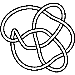
(KnotPlot image)	See the full Rolfsen Knot Table. Visit 9 40's page at the Knot Server (KnotPlot driven, includes 3D interactive images!) Visit 9 40 at Knotilus!

In three-fold symmetrical form		Symmetrical triangular form		(less open)		(alternate)		Variant
Obtained by an epitrochoid.		Cylindrical depiction.		9.40 as a geodesic line of the oblate spheroid		Photo of an alsatian chair, musée de l'oeuvre Notre Dame, Strasbourg, France.

Knot presentations

Planar diagram presentation	X1627 X7,12,8,13 X5,15,6,14 X11,3,12,2 X15,10,16,11 X3,16,4,17 X9,4,10,5 X17,9,18,8 X13,18,14,1
Gauss code	-1, 4, -6, 7, -3, 1, -2, 8, -7, 5, -4, 2, -9, 3, -5, 6, -8, 9
Dowker-Thistlethwaite code	6 16 14 12 4 2 18 10 8
Conway Notation	[9*]

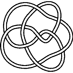
Minimum Braid Representative	A Morse Link Presentation	An Arc Presentation
Length is 9, width is 4, Braid index is 4		[{11, 3}, {2, 8}, {9, 4}, {3, 5}, {4, 1}, {7, 2}, {8, 6}, {10, 7}, {5, 9}, {6, 11}, {1, 10}]

[edit Notes on presentations of 9 40]

Computer Talk

The above data is available with the Mathematica package KnotTheory`. Your input (in red) is realistic; all else should have the same content as in a real mathematica session, but with different formatting.

(The path below may be different on your system, and possibly also the KnotTheory` date)

In[1]:=

AppendTo[$Path, "C:/drorbn/projects/KAtlas/"]; << KnotTheory`

Loading KnotTheory` version of May 31, 2006, 14:15:20.091. Read more at http://katlas.org/wiki/KnotTheory.

In[3]:=

K = Knot["9 40"];

In[4]:=

PD[K]

KnotTheory::loading: Loading precomputed data in PD4Knots`.

Out[4]=

X1627 X7,12,8,13 X5,15,6,14 X11,3,12,2 X15,10,16,11 X3,16,4,17 X9,4,10,5 X17,9,18,8 X13,18,14,1

In[5]:=

GaussCode[K]

Out[5]=

-1, 4, -6, 7, -3, 1, -2, 8, -7, 5, -4, 2, -9, 3, -5, 6, -8, 9

In[6]:=

DTCode[K]

Out[6]=

6 16 14 12 4 2 18 10 8

(The path below may be different on your system)

In[7]:=

AppendTo[$Path, "C:/bin/LinKnot/"];

In[8]:=

ConwayNotation[K]

Out[8]=

[9*]

In[9]:=

br = BR[K]

KnotTheory::credits: The minimum braids representing the knots with up to 10 crossings were provided by Thomas Gittings. See arXiv:math.GT/0401051.

Out[9]=

Failed to parse (SVG (MathML can be enabled via browser plugin): Invalid response ("Math extension cannot connect to Restbase.") from server "https://wikimedia.org/api/rest_v1/":): {\displaystyle \textrm{BR}(4,\{-1,2,-1,-3,2,-1,-3,2,-3\})}

In[10]:=

{First[br], Crossings[br], BraidIndex[K]}

KnotTheory::credits: The braid index data known to KnotTheory` is taken from Charles Livingston's http://www.indiana.edu/~knotinfo/.

KnotTheory::loading: Loading precomputed data in IndianaData`.

Out[10]=

{ 4, 9, 4 }

In[11]:=

Show[BraidPlot[br]]

Out[11]=

-Graphics-

In[12]:=

Show[DrawMorseLink[K]]

KnotTheory::credits: "MorseLink was added to KnotTheory` by Siddarth Sankaran at the University of Toronto in the summer of 2005."

KnotTheory::credits: "DrawMorseLink was written by Siddarth Sankaran at the University of Toronto in the summer of 2005."

Out[12]=

-Graphics-

In[13]:=

ap = ArcPresentation[K]

Out[13]=

ArcPresentation[{11, 3}, {2, 8}, {9, 4}, {3, 5}, {4, 1}, {7, 2}, {8, 6}, {10, 7}, {5, 9}, {6, 11}, {1, 10}]

In[14]:=

Draw[ap]

Out[14]=

-Graphics-

Three dimensional invariants

Symmetry type Reversible Unknotting number 2 3-genus 3 Bridge index 3 Super bridge index 4 Nakanishi index 2 Maximal Thurston-Bennequin number [-9][-2] Hyperbolic Volume 15.0183 A-Polynomial See Data:9 40/A-polynomial

[edit Notes for 9 40's three dimensional invariants]

Four dimensional invariants

Smooth 4 genus $1$ Topological 4 genus $1$ Concordance genus $[1,3]$ Rasmussen s-Invariant -2

[edit Notes for 9 40's four dimensional invariants]

Polynomial invariants

Alexander polynomial	$t^{3}-7t^{2}+18t-23+18t^{-1}-7t^{-2}+t^{-3}$
Conway polynomial	$z^{6}-z^{4}-z^{2}+1$
2nd Alexander ideal (db, data sources)	$\left\{t^{2}-3t+1\right\}$
Determinant and Signature	{ 75, -2 }
Jones polynomial	$-q^{2}+5q-8+11q^{-1}-13q^{-2}+13q^{-3}-11q^{-4}+8q^{-5}-4q^{-6}+q^{-7}$
HOMFLY-PT polynomial (db, data sources)	$z^{2}a^{6}-2z^{4}a^{4}-2z^{2}a^{4}+a^{4}+z^{6}a^{2}+2z^{4}a^{2}-2a^{2}-z^{4}+2$
Kauffman polynomial (db, data sources)	$z^{4}a^{8}+4z^{5}a^{7}-2z^{3}a^{7}+8z^{6}a^{6}-9z^{4}a^{6}+4z^{2}a^{6}+9z^{7}a^{5}-12z^{5}a^{5}+6z^{3}a^{5}-za^{5}+4z^{8}a^{4}+7z^{6}a^{4}-20z^{4}a^{4}+7z^{2}a^{4}+a^{4}+17z^{7}a^{3}-32z^{5}a^{3}+14z^{3}a^{3}-za^{3}+4z^{8}a^{2}+4z^{6}a^{2}-17z^{4}a^{2}+3z^{2}a^{2}+2a^{2}+8z^{7}a-15z^{5}a+6z^{3}a+5z^{6}-7z^{4}+2+z^{5}a^{-1}$
The A2 invariant	$q^{22}-q^{20}-2q^{18}+3q^{16}-q^{14}+2q^{12}+q^{10}-3q^{8}+q^{6}-4q^{4}+3q^{2}+1+3q^{-4}-q^{-6}$
The G2 invariant	$q^{114}-3q^{112}+6q^{110}-10q^{108}+10q^{106}-8q^{104}+q^{102}+17q^{100}-35q^{98}+57q^{96}-69q^{94}+58q^{92}-26q^{90}-41q^{88}+121q^{86}-182q^{84}+197q^{82}-139q^{80}+14q^{78}+135q^{76}-248q^{74}+274q^{72}-196q^{70}+38q^{68}+122q^{66}-223q^{64}+212q^{62}-79q^{60}-87q^{58}+218q^{56}-237q^{54}+135q^{52}+47q^{50}-232q^{48}+337q^{46}-328q^{44}+209q^{42}-7q^{40}-197q^{38}+334q^{36}-361q^{34}+269q^{32}-104q^{30}-93q^{28}+225q^{26}-263q^{24}+194q^{22}-39q^{20}-123q^{18}+217q^{16}-194q^{14}+58q^{12}+116q^{10}-252q^{8}+282q^{6}-192q^{4}+31q^{2}+141-245q^{-2}+261q^{-4}-179q^{-6}+57q^{-8}+53q^{-10}-121q^{-12}+126q^{-14}-87q^{-16}+44q^{-18}-2q^{-20}-19q^{-22}+24q^{-24}-20q^{-26}+10q^{-28}-4q^{-30}+q^{-32}$

Further Quantum Invariants

Further quantum knot invariants for 9_40.

A1 Invariants.

Weight	Invariant
1	$q^{15}-3q^{13}+4q^{11}-3q^{9}+2q^{7}-2q^{3}+3q-3q^{-1}+4q^{-3}-q^{-5}$
2	$q^{42}-3q^{40}+q^{38}+9q^{36}-16q^{34}-3q^{32}+33q^{30}-22q^{28}-22q^{26}+40q^{24}-8q^{22}-30q^{20}+20q^{18}+12q^{16}-17q^{14}-8q^{12}+23q^{10}+2q^{8}-31q^{6}+22q^{4}+22q^{2}-39+6q^{-2}+30q^{-4}-23q^{-6}-9q^{-8}+17q^{-10}-q^{-12}-4q^{-14}+q^{-16}$
3	$q^{81}-3q^{79}+q^{77}+6q^{75}-4q^{73}-15q^{71}+6q^{69}+47q^{67}-7q^{65}-96q^{63}-23q^{61}+150q^{59}+98q^{57}-188q^{55}-190q^{53}+175q^{51}+278q^{49}-113q^{47}-333q^{45}+25q^{43}+330q^{41}+63q^{39}-274q^{37}-133q^{35}+194q^{33}+176q^{31}-106q^{29}-195q^{27}+19q^{25}+205q^{23}+57q^{21}-209q^{19}-133q^{17}+203q^{15}+208q^{13}-176q^{11}-271q^{9}+115q^{7}+321q^{5}-34q^{3}-324q-59q^{-1}+279q^{-3}+139q^{-5}-192q^{-7}-173q^{-9}+96q^{-11}+153q^{-13}-16q^{-15}-102q^{-17}-28q^{-19}+52q^{-21}+24q^{-23}-11q^{-25}-13q^{-27}+q^{-29}+4q^{-31}-q^{-33}$
4	$q^{132}-3q^{130}+q^{128}+6q^{126}-7q^{124}-3q^{122}-6q^{120}+26q^{118}+38q^{116}-57q^{114}-83q^{112}-54q^{110}+169q^{108}+307q^{106}-58q^{104}-449q^{102}-561q^{100}+209q^{98}+1103q^{96}+687q^{94}-602q^{92}-1796q^{90}-834q^{88}+1520q^{86}+2270q^{84}+609q^{82}-2404q^{80}-2683q^{78}+308q^{76}+2944q^{74}+2520q^{72}-1207q^{70}-3340q^{68}-1547q^{66}+1770q^{64}+3142q^{62}+602q^{60}-2211q^{58}-2299q^{56}+53q^{54}+2248q^{52}+1548q^{50}-641q^{48}-1962q^{46}-1023q^{44}+1075q^{42}+1812q^{40}+483q^{38}-1542q^{36}-1702q^{34}+205q^{32}+2090q^{30}+1450q^{28}-1214q^{26}-2450q^{24}-829q^{22}+2208q^{20}+2605q^{18}-303q^{16}-2836q^{14}-2279q^{12}+1320q^{10}+3252q^{8}+1350q^{6}-1886q^{4}-3163q^{2}-544+2305q^{-2}+2419q^{-4}+110q^{-6}-2297q^{-8}-1724q^{-10}+331q^{-12}+1714q^{-14}+1253q^{-16}-522q^{-18}-1171q^{-20}-683q^{-22}+324q^{-24}+800q^{-26}+287q^{-28}-187q^{-30}-393q^{-32}-164q^{-34}+136q^{-36}+134q^{-38}+65q^{-40}-44q^{-42}-53q^{-44}-4q^{-46}+7q^{-48}+13q^{-50}-q^{-52}-4q^{-54}+q^{-56}$
5	$q^{195}-3q^{193}+q^{191}+6q^{189}-7q^{187}-6q^{185}+6q^{183}+14q^{181}+17q^{179}-6q^{177}-68q^{175}-90q^{173}+31q^{171}+223q^{169}+281q^{167}+9q^{165}-504q^{163}-829q^{161}-385q^{159}+910q^{157}+1976q^{155}+1479q^{153}-919q^{151}-3669q^{149}-3993q^{147}-320q^{145}+5365q^{143}+7993q^{141}+3795q^{139}-5578q^{137}-12701q^{135}-10047q^{133}+2784q^{131}+16391q^{129}+18101q^{127}+3797q^{125}-16705q^{123}-25866q^{121}-13539q^{119}+12444q^{117}+30646q^{115}+24001q^{113}-3906q^{111}-30412q^{109}-32341q^{107}-6868q^{105}+25059q^{103}+36221q^{101}+16940q^{99}-16089q^{97}-34824q^{95}-23986q^{93}+5996q^{91}+29197q^{89}+26869q^{87}+2813q^{85}-21320q^{83}-25896q^{81}-9071q^{79}+13300q^{77}+22554q^{75}+12559q^{73}-6644q^{71}-18493q^{69}-13997q^{67}+1817q^{65}+15043q^{63}+14672q^{61}+1434q^{59}-12928q^{57}-15598q^{55}-3914q^{53}+11985q^{51}+17517q^{49}+6674q^{47}-11643q^{45}-20517q^{43}-10461q^{41}+10796q^{39}+23989q^{37}+15718q^{35}-8296q^{33}-26901q^{31}-22122q^{29}+3419q^{27}+27710q^{25}+28570q^{23}+4041q^{21}-25170q^{19}-33454q^{17}-13019q^{15}+18728q^{13}+34795q^{11}+21734q^{9}-9014q^{7}-31506q^{5}-27744q^{3}-2006q+23734q^{-1}+29144q^{-3}+11595q^{-5}-13164q^{-7}-25450q^{-9}-17354q^{-11}+2643q^{-13}+17992q^{-15}+18081q^{-17}+5151q^{-19}-9254q^{-21}-14599q^{-23}-8790q^{-25}+1983q^{-27}+9097q^{-29}+8440q^{-31}+2256q^{-33}-3848q^{-35}-5856q^{-37}-3509q^{-39}+517q^{-41}+2960q^{-43}+2723q^{-45}+860q^{-47}-888q^{-49}-1496q^{-51}-918q^{-53}+30q^{-55}+527q^{-57}+501q^{-59}+179q^{-61}-102q^{-63}-195q^{-65}-107q^{-67}+7q^{-69}+45q^{-71}+33q^{-73}+8q^{-75}-7q^{-77}-13q^{-79}+q^{-81}+4q^{-83}-q^{-85}$

A2 Invariants.

Weight	Invariant
1,0	Failed to parse (SVG (MathML can be enabled via browser plugin): Invalid response ("Math extension cannot connect to Restbase.") from server "https://wikimedia.org/api/rest_v1/":): {\displaystyle q^{22}-q^{20}-2 q^{18}+3 q^{16}-q^{14}+2 q^{12}+q^{10}-3 q^8+q^6-4 q^4+3 q^2+1+3 q^{-4} - q^{-6} }
1,1	Failed to parse (SVG (MathML can be enabled via browser plugin): Invalid response ("Math extension cannot connect to Restbase.") from server "https://wikimedia.org/api/rest_v1/":): {\displaystyle q^{60}-6 q^{58}+18 q^{56}-38 q^{54}+75 q^{52}-144 q^{50}+244 q^{48}-382 q^{46}+576 q^{44}-798 q^{42}+1004 q^{40}-1168 q^{38}+1223 q^{36}-1110 q^{34}+828 q^{32}-360 q^{30}-236 q^{28}+880 q^{26}-1502 q^{24}+1988 q^{22}-2316 q^{20}+2426 q^{18}-2296 q^{16}+1966 q^{14}-1452 q^{12}+850 q^{10}-198 q^8-408 q^6+885 q^4-1194 q^2+1304-1250 q^{-2} +1061 q^{-4} -814 q^{-6} +568 q^{-8} -338 q^{-10} +184 q^{-12} -88 q^{-14} +32 q^{-16} -8 q^{-18} + q^{-20} }
2,0	Failed to parse (SVG (MathML can be enabled via browser plugin): Invalid response ("Math extension cannot connect to Restbase.") from server "https://wikimedia.org/api/rest_v1/":): {\displaystyle q^{56}-q^{54}-3 q^{52}+2 q^{50}+6 q^{48}-q^{46}-11 q^{44}-q^{42}+16 q^{40}-3 q^{38}-13 q^{36}+6 q^{34}+16 q^{32}-3 q^{30}-19 q^{28}+7 q^{26}+4 q^{24}-12 q^{22}-q^{20}+8 q^{18}-2 q^{16}+16 q^{12}-12 q^8+2 q^6+14 q^4-10 q^2-18+12 q^{-2} +10 q^{-4} -8 q^{-6} -6 q^{-8} +6 q^{-10} +9 q^{-12} -3 q^{-14} -3 q^{-16} + q^{-18} }

A3 Invariants.

Weight	Invariant
0,1,0	Failed to parse (SVG (MathML can be enabled via browser plugin): Invalid response ("Math extension cannot connect to Restbase.") from server "https://wikimedia.org/api/rest_v1/":): {\displaystyle q^{48}-3 q^{46}+9 q^{42}-10 q^{40}-4 q^{38}+22 q^{36}-19 q^{34}-10 q^{32}+29 q^{30}-20 q^{28}-8 q^{26}+24 q^{24}-7 q^{22}-6 q^{20}+5 q^{18}+7 q^{16}-4 q^{14}-15 q^{12}+13 q^{10}+7 q^8-28 q^6+15 q^4+15 q^2-26+16 q^{-2} +10 q^{-4} -15 q^{-6} +9 q^{-8} +2 q^{-10} -4 q^{-12} + q^{-14} }
1,0,0	Failed to parse (SVG (MathML can be enabled via browser plugin): Invalid response ("Math extension cannot connect to Restbase.") from server "https://wikimedia.org/api/rest_v1/":): {\displaystyle q^{29}-q^{27}-2 q^{23}+3 q^{21}-2 q^{19}+4 q^{17}+q^{13}-2 q^{11}-2 q^9-q^7-3 q^5+3 q^3+4 q^{-1} - q^{-3} +3 q^{-5} - q^{-7} }

A4 Invariants.

Weight	Invariant
0,1,0,0	Failed to parse (SVG (MathML can be enabled via browser plugin): Invalid response ("Math extension cannot connect to Restbase.") from server "https://wikimedia.org/api/rest_v1/":): {\displaystyle q^{62}-q^{60}-3 q^{58}+q^{56}+6 q^{54}+q^{52}-10 q^{50}+2 q^{48}+15 q^{46}-9 q^{44}-19 q^{42}+16 q^{40}+13 q^{38}-21 q^{36}-6 q^{34}+23 q^{32}-21 q^{28}+13 q^{26}+18 q^{24}-20 q^{22}-4 q^{20}+29 q^{18}-12 q^{16}-23 q^{14}+20 q^{12}+8 q^{10}-28 q^8-8 q^6+21 q^4-15+11 q^{-2} +17 q^{-4} -6 q^{-6} -4 q^{-8} +8 q^{-10} - q^{-12} -3 q^{-14} + q^{-16} }
1,0,0,0	Failed to parse (SVG (MathML can be enabled via browser plugin): Invalid response ("Math extension cannot connect to Restbase.") from server "https://wikimedia.org/api/rest_v1/":): {\displaystyle q^{36}-q^{34}-2 q^{28}+3 q^{26}-2 q^{24}+3 q^{22}+2 q^{20}+q^{16}-2 q^{14}-q^{12}-4 q^{10}-3 q^6+3 q^4+3+3 q^{-2} - q^{-4} +3 q^{-6} - q^{-8} }

B2 Invariants.

Weight	Invariant
0,1	$q^{48}-3q^{46}+6q^{44}-11q^{42}+18q^{40}-24q^{38}+30q^{36}-33q^{34}+28q^{32}-21q^{30}+10q^{28}+4q^{26}-18q^{24}+37q^{22}-48q^{20}+57q^{18}-59q^{16}+54q^{14}-47q^{12}+31q^{10}-17q^{8}-2q^{6}+15q^{4}-23q^{2}+30-30q^{-2}+32q^{-4}-23q^{-6}+17q^{-8}-10q^{-10}+4q^{-12}-q^{-14}$
1,0	Failed to parse (SVG (MathML can be enabled via browser plugin): Invalid response ("Math extension cannot connect to Restbase.") from server "https://wikimedia.org/api/rest_v1/":): {\displaystyle q^{78}-3 q^{74}-3 q^{72}+3 q^{70}+10 q^{68}+3 q^{66}-14 q^{64}-14 q^{62}+9 q^{60}+26 q^{58}+4 q^{56}-31 q^{54}-19 q^{52}+22 q^{50}+29 q^{48}-9 q^{46}-32 q^{44}-2 q^{42}+29 q^{40}+12 q^{38}-23 q^{36}-14 q^{34}+17 q^{32}+18 q^{30}-11 q^{28}-21 q^{26}+6 q^{24}+21 q^{22}-q^{20}-23 q^{18}-5 q^{16}+24 q^{14}+15 q^{12}-24 q^{10}-27 q^8+15 q^6+34 q^4-32-15 q^{-2} +23 q^{-4} +25 q^{-6} -10 q^{-8} -19 q^{-10} - q^{-12} +13 q^{-14} +6 q^{-16} -4 q^{-18} -4 q^{-20} + q^{-24} }

D4 Invariants.

Weight

Invariant

1,0,0,0

Failed to parse (SVG (MathML can be enabled via browser plugin): Invalid response ("Math extension cannot connect to Restbase.") from server "https://wikimedia.org/api/rest_v1/":): {\displaystyle q^{66}-3 q^{64}+3 q^{62}-4 q^{60}+10 q^{58}-14 q^{56}+14 q^{54}-17 q^{52}+26 q^{50}-27 q^{48}+21 q^{46}-23 q^{44}+20 q^{42}-11 q^{40}+2 q^{38}+q^{36}-10 q^{34}+28 q^{32}-29 q^{30}+36 q^{28}-41 q^{26}+48 q^{24}-43 q^{22}+40 q^{20}-43 q^{18}+30 q^{16}-24 q^{14}+14 q^{12}-12 q^{10}-4 q^8+14 q^6-15 q^4+21 q^2-22+29 q^{-2} -22 q^{-4} +24 q^{-6} -19 q^{-8} +14 q^{-10} -8 q^{-12} +6 q^{-14} -4 q^{-16} + q^{-18} }

G2 Invariants.

Weight

Invariant

1,0

Failed to parse (SVG (MathML can be enabled via browser plugin): Invalid response ("Math extension cannot connect to Restbase.") from server "https://wikimedia.org/api/rest_v1/":): {\displaystyle q^{114}-3 q^{112}+6 q^{110}-10 q^{108}+10 q^{106}-8 q^{104}+q^{102}+17 q^{100}-35 q^{98}+57 q^{96}-69 q^{94}+58 q^{92}-26 q^{90}-41 q^{88}+121 q^{86}-182 q^{84}+197 q^{82}-139 q^{80}+14 q^{78}+135 q^{76}-248 q^{74}+274 q^{72}-196 q^{70}+38 q^{68}+122 q^{66}-223 q^{64}+212 q^{62}-79 q^{60}-87 q^{58}+218 q^{56}-237 q^{54}+135 q^{52}+47 q^{50}-232 q^{48}+337 q^{46}-328 q^{44}+209 q^{42}-7 q^{40}-197 q^{38}+334 q^{36}-361 q^{34}+269 q^{32}-104 q^{30}-93 q^{28}+225 q^{26}-263 q^{24}+194 q^{22}-39 q^{20}-123 q^{18}+217 q^{16}-194 q^{14}+58 q^{12}+116 q^{10}-252 q^8+282 q^6-192 q^4+31 q^2+141-245 q^{-2} +261 q^{-4} -179 q^{-6} +57 q^{-8} +53 q^{-10} -121 q^{-12} +126 q^{-14} -87 q^{-16} +44 q^{-18} -2 q^{-20} -19 q^{-22} +24 q^{-24} -20 q^{-26} +10 q^{-28} -4 q^{-30} + q^{-32} }

.

Computer Talk

The above data is available with the Mathematica package KnotTheory`, as shown in the (simulated) Mathematica session below. Your input (in red) is realistic; all else should have the same content as in a real mathematica session, but with different formatting. This Mathematica session is also available (albeit only for the knot 5_2) as the notebook PolynomialInvariantsSession.nb.

(The path below may be different on your system, and possibly also the KnotTheory` date)

In[1]:=

AppendTo[$Path, "C:/drorbn/projects/KAtlas/"]; << KnotTheory`

Loading KnotTheory` version of August 31, 2006, 11:25:27.5625. Read more at http://katlas.math.toronto.edu/wiki/KnotTheory.

In[3]:=

K = Knot["9 40"];

In[4]:=

Alexander[K][t]

KnotTheory::loading: Loading precomputed data in PD4Knots`.

Out[4]=

$t^{3}-7t^{2}+18t-23+18t^{-1}-7t^{-2}+t^{-3}$

In[5]:=

Conway[K][z]

Out[5]=

$z^{6}-z^{4}-z^{2}+1$

In[6]:=

Alexander[K, 2][t]

KnotTheory::credits: The program Alexander[K, r] to compute Alexander ideals was written by Jana Archibald at the University of Toronto in the summer of 2005.

Out[6]=

$\left\{t^{2}-3t+1\right\}$

In[7]:=

{KnotDet[K], KnotSignature[K]}

Out[7]=

{ 75, -2 }

In[8]:=

Jones[K][q]

KnotTheory::loading: Loading precomputed data in Jones4Knots`.

Out[8]=

$-q^{2}+5q-8+11q^{-1}-13q^{-2}+13q^{-3}-11q^{-4}+8q^{-5}-4q^{-6}+q^{-7}$

In[9]:=

HOMFLYPT[K][a, z]

KnotTheory::credits: The HOMFLYPT program was written by Scott Morrison.

Out[9]=

$z^{2}a^{6}-2z^{4}a^{4}-2z^{2}a^{4}+a^{4}+z^{6}a^{2}+2z^{4}a^{2}-2a^{2}-z^{4}+2$

In[10]:=

Kauffman[K][a, z]

KnotTheory::loading: Loading precomputed data in Kauffman4Knots`.

Out[10]=

$z^{4}a^{8}+4z^{5}a^{7}-2z^{3}a^{7}+8z^{6}a^{6}-9z^{4}a^{6}+4z^{2}a^{6}+9z^{7}a^{5}-12z^{5}a^{5}+6z^{3}a^{5}-za^{5}+4z^{8}a^{4}+7z^{6}a^{4}-20z^{4}a^{4}+7z^{2}a^{4}+a^{4}+17z^{7}a^{3}-32z^{5}a^{3}+14z^{3}a^{3}-za^{3}+4z^{8}a^{2}+4z^{6}a^{2}-17z^{4}a^{2}+3z^{2}a^{2}+2a^{2}+8z^{7}a-15z^{5}a+6z^{3}a+5z^{6}-7z^{4}+2+z^{5}a^{-1}$

"Similar" Knots (within the Atlas)

Same Alexander/Conway Polynomial: {10_59, K11n66,}

Same Jones Polynomial (up to mirroring, Failed to parse (SVG (MathML can be enabled via browser plugin): Invalid response ("Math extension cannot connect to Restbase.") from server "https://wikimedia.org/api/rest_v1/":): {\displaystyle q\leftrightarrow q^{-1}} ): {}

Computer Talk

The above data is available with the Mathematica package KnotTheory`. Your input (in red) is realistic; all else should have the same content as in a real mathematica session, but with different formatting.

(The path below may be different on your system, and possibly also the KnotTheory` date)

In[1]:=

AppendTo[$Path, "C:/drorbn/projects/KAtlas/"]; << KnotTheory`

Loading KnotTheory` version of May 31, 2006, 14:15:20.091. Read more at http://katlas.math.toronto.edu/wiki/KnotTheory.

In[3]:=

K = Knot["9 40"];

In[4]:=

{A = Alexander[K][t], J = Jones[K][q]}

KnotTheory::loading: Loading precomputed data in PD4Knots`.

KnotTheory::loading: Loading precomputed data in Jones4Knots`.

Out[4]=

{ Failed to parse (SVG (MathML can be enabled via browser plugin): Invalid response ("Math extension cannot connect to Restbase.") from server "https://wikimedia.org/api/rest_v1/":): {\displaystyle t^3-7 t^2+18 t-23+18 t^{-1} -7 t^{-2} + t^{-3} } , Failed to parse (SVG (MathML can be enabled via browser plugin): Invalid response ("Math extension cannot connect to Restbase.") from server "https://wikimedia.org/api/rest_v1/":): {\displaystyle -q^2+5 q-8+11 q^{-1} -13 q^{-2} +13 q^{-3} -11 q^{-4} +8 q^{-5} -4 q^{-6} + q^{-7} } }

In[5]:=

DeleteCases[Select[AllKnots[], (A === Alexander[#][t]) &], K]

KnotTheory::loading: Loading precomputed data in DTCode4KnotsTo11`.

KnotTheory::credits: The GaussCode to PD conversion was written by Siddarth Sankaran at the University of Toronto in the summer of 2005.

Out[5]=

{10_59, K11n66,}

In[6]:=

DeleteCases[ Select[ AllKnots[], (J === Jones[#][q] || (J /. q -> 1/q) === Jones[#][q]) & ], K ]

KnotTheory::loading: Loading precomputed data in Jones4Knots11`.

Out[6]=

{}

Vassiliev invariants

V2 and V3:

(-1, 1)

V2,1 through V6,9:

V2,1 V3,1 V4,1 V4,2 V4,3 V5,1 V5,2 V5,3 V5,4 V6,1 V6,2 V6,3 V6,4 V6,5 V6,6 V6,7 V6,8 V6,9 Failed to parse (SVG (MathML can be enabled via browser plugin): Invalid response ("Math extension cannot connect to Restbase.") from server "https://wikimedia.org/api/rest_v1/":): {\displaystyle -4} Failed to parse (SVG (MathML can be enabled via browser plugin): Invalid response ("Math extension cannot connect to Restbase.") from server "https://wikimedia.org/api/rest_v1/":): {\displaystyle 8} $8$ Failed to parse (SVG (MathML can be enabled via browser plugin): Invalid response ("Math extension cannot connect to Restbase.") from server "https://wikimedia.org/api/rest_v1/":): {\displaystyle \frac{34}{3}} Failed to parse (SVG (MathML can be enabled via browser plugin): Invalid response ("Math extension cannot connect to Restbase.") from server "https://wikimedia.org/api/rest_v1/":): {\displaystyle \frac{38}{3}} Failed to parse (SVG (MathML can be enabled via browser plugin): Invalid response ("Math extension cannot connect to Restbase.") from server "https://wikimedia.org/api/rest_v1/":): {\displaystyle -32} Failed to parse (SVG (MathML can be enabled via browser plugin): Invalid response ("Math extension cannot connect to Restbase.") from server "https://wikimedia.org/api/rest_v1/":): {\displaystyle -\frac{208}{3}} Failed to parse (SVG (MathML can be enabled via browser plugin): Invalid response ("Math extension cannot connect to Restbase.") from server "https://wikimedia.org/api/rest_v1/":): {\displaystyle -\frac{160}{3}} Failed to parse (SVG (MathML can be enabled via browser plugin): Invalid response ("Math extension cannot connect to Restbase.") from server "https://wikimedia.org/api/rest_v1/":): {\displaystyle 8} Failed to parse (SVG (MathML can be enabled via browser plugin): Invalid response ("Math extension cannot connect to Restbase.") from server "https://wikimedia.org/api/rest_v1/":): {\displaystyle -\frac{32}{3}} Failed to parse (SVG (MathML can be enabled via browser plugin): Invalid response ("Math extension cannot connect to Restbase.") from server "https://wikimedia.org/api/rest_v1/":): {\displaystyle 32} $-{\frac {136}{3}}$ Failed to parse (SVG (MathML can be enabled via browser plugin): Invalid response ("Math extension cannot connect to Restbase.") from server "https://wikimedia.org/api/rest_v1/":): {\displaystyle -\frac{152}{3}} Failed to parse (SVG (MathML can be enabled via browser plugin): Invalid response ("Math extension cannot connect to Restbase.") from server "https://wikimedia.org/api/rest_v1/":): {\displaystyle \frac{2129}{30}} Failed to parse (SVG (MathML can be enabled via browser plugin): Invalid response ("Math extension cannot connect to Restbase.") from server "https://wikimedia.org/api/rest_v1/":): {\displaystyle \frac{2102}{15}} Failed to parse (SVG (MathML can be enabled via browser plugin): Invalid response ("Math extension cannot connect to Restbase.") from server "https://wikimedia.org/api/rest_v1/":): {\displaystyle -\frac{4742}{45}} Failed to parse (SVG (MathML can be enabled via browser plugin): Invalid response ("Math extension cannot connect to Restbase.") from server "https://wikimedia.org/api/rest_v1/":): {\displaystyle -\frac{113}{18}} Failed to parse (SVG (MathML can be enabled via browser plugin): Invalid response ("Math extension cannot connect to Restbase.") from server "https://wikimedia.org/api/rest_v1/":): {\displaystyle -\frac{751}{30}}

V_2,1 through V_6,9 were provided by Petr Dunin-Barkowski <barkovs@itep.ru>, Andrey Smirnov <asmirnov@itep.ru>, and Alexei Sleptsov <sleptsov@itep.ru> and uploaded on October 2010 by User:Drorbn. Note that they are normalized differently than V₂ and V₃.

Khovanov Homology

The coefficients of the monomials Failed to parse (SVG (MathML can be enabled via browser plugin): Invalid response ("Math extension cannot connect to Restbase.") from server "https://wikimedia.org/api/rest_v1/":): {\displaystyle t^rq^j} are shown, along with their alternating sums Failed to parse (SVG (MathML can be enabled via browser plugin): Invalid response ("Math extension cannot connect to Restbase.") from server "https://wikimedia.org/api/rest_v1/":): {\displaystyle \chi} (fixed Failed to parse (SVG (MathML can be enabled via browser plugin): Invalid response ("Math extension cannot connect to Restbase.") from server "https://wikimedia.org/api/rest_v1/":): {\displaystyle j} , alternation over Failed to parse (SVG (MathML can be enabled via browser plugin): Invalid response ("Math extension cannot connect to Restbase.") from server "https://wikimedia.org/api/rest_v1/":): {\displaystyle r} ). The squares with yellow highlighting are those on the "critical diagonals", where Failed to parse (SVG (MathML can be enabled via browser plugin): Invalid response ("Math extension cannot connect to Restbase.") from server "https://wikimedia.org/api/rest_v1/":): {\displaystyle j-2r=s+1} or Failed to parse (SVG (MathML can be enabled via browser plugin): Invalid response ("Math extension cannot connect to Restbase.") from server "https://wikimedia.org/api/rest_v1/":): {\displaystyle j-2r=s-1} , where Failed to parse (SVG (MathML can be enabled via browser plugin): Invalid response ("Math extension cannot connect to Restbase.") from server "https://wikimedia.org/api/rest_v1/":): {\displaystyle s=} -2 is the signature of 9 40. Nonzero entries off the critical diagonals (if any exist) are highlighted in red.

\   r    \    j   \ -6 -5 -4 -3 -2 -1 0 1 2 3 χ 5                   1 -1 3                 4   4 1               4 1   -3 -1             7 4     3 -3           7 5       -2 -5         6 6         0 -7       5 7           2 -9     3 6             -3 -11   1 5               4 -13   3                 -3 -15 1                   1

Integral Khovanov Homology (db, data source)

Failed to parse (SVG (MathML can be enabled via browser plugin): Invalid response ("Math extension cannot connect to Restbase.") from server "https://wikimedia.org/api/rest_v1/":): {\displaystyle \dim{\mathcal G}_{2r+i}\operatorname{KH}^r_{\mathbb Z}} Failed to parse (SVG (MathML can be enabled via browser plugin): Invalid response ("Math extension cannot connect to Restbase.") from server "https://wikimedia.org/api/rest_v1/":): {\displaystyle i=-3} $i=-1$ $r=-6$ Failed to parse (SVG (MathML can be enabled via browser plugin): Invalid response ("Math extension cannot connect to Restbase.") from server "https://wikimedia.org/api/rest_v1/":): {\displaystyle {\mathbb Z}} Failed to parse (SVG (MathML can be enabled via browser plugin): Invalid response ("Math extension cannot connect to Restbase.") from server "https://wikimedia.org/api/rest_v1/":): {\displaystyle r=-5} Failed to parse (SVG (MathML can be enabled via browser plugin): Invalid response ("Math extension cannot connect to Restbase.") from server "https://wikimedia.org/api/rest_v1/":): {\displaystyle {\mathbb Z}^{3}\oplus{\mathbb Z}_2} Failed to parse (SVG (MathML can be enabled via browser plugin): Invalid response ("Math extension cannot connect to Restbase.") from server "https://wikimedia.org/api/rest_v1/":): {\displaystyle {\mathbb Z}} Failed to parse (SVG (MathML can be enabled via browser plugin): Invalid response ("Math extension cannot connect to Restbase.") from server "https://wikimedia.org/api/rest_v1/":): {\displaystyle r=-4} Failed to parse (SVG (MathML can be enabled via browser plugin): Invalid response ("Math extension cannot connect to Restbase.") from server "https://wikimedia.org/api/rest_v1/":): {\displaystyle {\mathbb Z}^{5}\oplus{\mathbb Z}_2^{3}} Failed to parse (SVG (MathML can be enabled via browser plugin): Invalid response ("Math extension cannot connect to Restbase.") from server "https://wikimedia.org/api/rest_v1/":): {\displaystyle {\mathbb Z}^{3}} Failed to parse (SVG (MathML can be enabled via browser plugin): Invalid response ("Math extension cannot connect to Restbase.") from server "https://wikimedia.org/api/rest_v1/":): {\displaystyle r=-3} Failed to parse (SVG (MathML can be enabled via browser plugin): Invalid response ("Math extension cannot connect to Restbase.") from server "https://wikimedia.org/api/rest_v1/":): {\displaystyle {\mathbb Z}^{6}\oplus{\mathbb Z}_2^{5}} Failed to parse (SVG (MathML can be enabled via browser plugin): Invalid response ("Math extension cannot connect to Restbase.") from server "https://wikimedia.org/api/rest_v1/":): {\displaystyle {\mathbb Z}^{5}} Failed to parse (SVG (MathML can be enabled via browser plugin): Invalid response ("Math extension cannot connect to Restbase.") from server "https://wikimedia.org/api/rest_v1/":): {\displaystyle r=-2} Failed to parse (SVG (MathML can be enabled via browser plugin): Invalid response ("Math extension cannot connect to Restbase.") from server "https://wikimedia.org/api/rest_v1/":): {\displaystyle {\mathbb Z}^{7}\oplus{\mathbb Z}_2^{6}} Failed to parse (SVG (MathML can be enabled via browser plugin): Invalid response ("Math extension cannot connect to Restbase.") from server "https://wikimedia.org/api/rest_v1/":): {\displaystyle {\mathbb Z}^{6}} Failed to parse (SVG (MathML can be enabled via browser plugin): Invalid response ("Math extension cannot connect to Restbase.") from server "https://wikimedia.org/api/rest_v1/":): {\displaystyle r=-1} Failed to parse (SVG (MathML can be enabled via browser plugin): Invalid response ("Math extension cannot connect to Restbase.") from server "https://wikimedia.org/api/rest_v1/":): {\displaystyle {\mathbb Z}^{6}\oplus{\mathbb Z}_2^{7}} Failed to parse (SVG (MathML can be enabled via browser plugin): Invalid response ("Math extension cannot connect to Restbase.") from server "https://wikimedia.org/api/rest_v1/":): {\displaystyle {\mathbb Z}^{7}} Failed to parse (SVG (MathML can be enabled via browser plugin): Invalid response ("Math extension cannot connect to Restbase.") from server "https://wikimedia.org/api/rest_v1/":): {\displaystyle r=0} Failed to parse (SVG (MathML can be enabled via browser plugin): Invalid response ("Math extension cannot connect to Restbase.") from server "https://wikimedia.org/api/rest_v1/":): {\displaystyle {\mathbb Z}^{5}\oplus{\mathbb Z}_2^{6}} Failed to parse (SVG (MathML can be enabled via browser plugin): Invalid response ("Math extension cannot connect to Restbase.") from server "https://wikimedia.org/api/rest_v1/":): {\displaystyle {\mathbb Z}^{7}} Failed to parse (SVG (MathML can be enabled via browser plugin): Invalid response ("Math extension cannot connect to Restbase.") from server "https://wikimedia.org/api/rest_v1/":): {\displaystyle r=1} Failed to parse (SVG (MathML can be enabled via browser plugin): Invalid response ("Math extension cannot connect to Restbase.") from server "https://wikimedia.org/api/rest_v1/":): {\displaystyle {\mathbb Z}^{4}\oplus{\mathbb Z}_2^{4}} Failed to parse (SVG (MathML can be enabled via browser plugin): Invalid response ("Math extension cannot connect to Restbase.") from server "https://wikimedia.org/api/rest_v1/":): {\displaystyle {\mathbb Z}^{4}} Failed to parse (SVG (MathML can be enabled via browser plugin): Invalid response ("Math extension cannot connect to Restbase.") from server "https://wikimedia.org/api/rest_v1/":): {\displaystyle r=2} Failed to parse (SVG (MathML can be enabled via browser plugin): Invalid response ("Math extension cannot connect to Restbase.") from server "https://wikimedia.org/api/rest_v1/":): {\displaystyle {\mathbb Z}\oplus{\mathbb Z}_2^{4}} Failed to parse (SVG (MathML can be enabled via browser plugin): Invalid response ("Math extension cannot connect to Restbase.") from server "https://wikimedia.org/api/rest_v1/":): {\displaystyle {\mathbb Z}^{4}} Failed to parse (SVG (MathML can be enabled via browser plugin): Invalid response ("Math extension cannot connect to Restbase.") from server "https://wikimedia.org/api/rest_v1/":): {\displaystyle r=3} Failed to parse (SVG (MathML can be enabled via browser plugin): Invalid response ("Math extension cannot connect to Restbase.") from server "https://wikimedia.org/api/rest_v1/":): {\displaystyle {\mathbb Z}_2} Failed to parse (SVG (MathML can be enabled via browser plugin): Invalid response ("Math extension cannot connect to Restbase.") from server "https://wikimedia.org/api/rest_v1/":): {\displaystyle {\mathbb Z}}

The Coloured Jones Polynomials

The Coloured Jones Polynomials (in the Failed to parse (SVG (MathML can be enabled via browser plugin): Invalid response ("Math extension cannot connect to Restbase.") from server "https://wikimedia.org/api/rest_v1/":): {\displaystyle n+1} -dimensional representation of Failed to parse (SVG (MathML can be enabled via browser plugin): Invalid response ("Math extension cannot connect to Restbase.") from server "https://wikimedia.org/api/rest_v1/":): {\displaystyle sl(2)} )

Failed to parse (SVG (MathML can be enabled via browser plugin): Invalid response ("Math extension cannot connect to Restbase.") from server "https://wikimedia.org/api/rest_v1/":): {\displaystyle n}	Failed to parse (SVG (MathML can be enabled via browser plugin): Invalid response ("Math extension cannot connect to Restbase.") from server "https://wikimedia.org/api/rest_v1/":): {\displaystyle J_n}
2	Failed to parse (SVG (MathML can be enabled via browser plugin): Invalid response ("Math extension cannot connect to Restbase.") from server "https://wikimedia.org/api/rest_v1/":): {\displaystyle q^7-5 q^6+3 q^5+19 q^4-31 q^3-11 q^2+72 q-55-56 q^{-1} +133 q^{-2} -55 q^{-3} -109 q^{-4} +166 q^{-5} -34 q^{-6} -140 q^{-7} +157 q^{-8} -5 q^{-9} -132 q^{-10} +107 q^{-11} +17 q^{-12} -84 q^{-13} +45 q^{-14} +17 q^{-15} -29 q^{-16} +9 q^{-17} +4 q^{-18} -4 q^{-19} + q^{-20} }
3	Failed to parse (SVG (MathML can be enabled via browser plugin): Invalid response ("Math extension cannot connect to Restbase.") from server "https://wikimedia.org/api/rest_v1/":): {\displaystyle -q^{15}+5 q^{14}-3 q^{13}-14 q^{12}+q^{11}+40 q^{10}+25 q^9-94 q^8-73 q^7+126 q^6+194 q^5-151 q^4-342 q^3+107 q^2+525 q-11-680 q^{-1} -158 q^{-2} +815 q^{-3} +344 q^{-4} -886 q^{-5} -544 q^{-6} +910 q^{-7} +728 q^{-8} -891 q^{-9} -880 q^{-10} +834 q^{-11} +994 q^{-12} -743 q^{-13} -1066 q^{-14} +620 q^{-15} +1083 q^{-16} -461 q^{-17} -1048 q^{-18} +293 q^{-19} +942 q^{-20} -124 q^{-21} -781 q^{-22} -12 q^{-23} +584 q^{-24} +96 q^{-25} -390 q^{-26} -115 q^{-27} +219 q^{-28} +98 q^{-29} -104 q^{-30} -63 q^{-31} +46 q^{-32} +25 q^{-33} -15 q^{-34} -9 q^{-35} +5 q^{-36} +4 q^{-37} -4 q^{-38} + q^{-39} }
4	Failed to parse (SVG (MathML can be enabled via browser plugin): Invalid response ("Math extension cannot connect to Restbase.") from server "https://wikimedia.org/api/rest_v1/":): {\displaystyle q^{26}-5 q^{25}+3 q^{24}+14 q^{23}-6 q^{22}-10 q^{21}-54 q^{20}+12 q^{19}+123 q^{18}+63 q^{17}-8 q^{16}-354 q^{15}-217 q^{14}+329 q^{13}+537 q^{12}+505 q^{11}-830 q^{10}-1224 q^9-159 q^8+1186 q^7+2280 q^6-369 q^5-2607 q^4-2214 q^3+613 q^2+4687 q+1940-2721 q^{-1} -5063 q^{-2} -2006 q^{-3} +5964 q^{-4} +5176 q^{-5} -819 q^{-6} -6995 q^{-7} -5605 q^{-8} +5407 q^{-9} +7709 q^{-10} +2089 q^{-11} -7392 q^{-12} -8642 q^{-13} +3786 q^{-14} +8945 q^{-15} +4753 q^{-16} -6752 q^{-17} -10527 q^{-18} +1879 q^{-19} +9105 q^{-20} +6778 q^{-21} -5423 q^{-22} -11264 q^{-23} -219 q^{-24} +8166 q^{-25} +8099 q^{-26} -3234 q^{-27} -10564 q^{-28} -2414 q^{-29} +5814 q^{-30} +8187 q^{-31} -421 q^{-32} -8024 q^{-33} -3786 q^{-34} +2497 q^{-35} +6394 q^{-36} +1712 q^{-37} -4297 q^{-38} -3362 q^{-39} -139 q^{-40} +3403 q^{-41} +1991 q^{-42} -1284 q^{-43} -1701 q^{-44} -889 q^{-45} +1049 q^{-46} +1029 q^{-47} -90 q^{-48} -412 q^{-49} -473 q^{-50} +155 q^{-51} +259 q^{-52} +22 q^{-53} -21 q^{-54} -108 q^{-55} +17 q^{-56} +36 q^{-57} -7 q^{-58} +5 q^{-59} -13 q^{-60} +5 q^{-61} +4 q^{-62} -4 q^{-63} + q^{-64} }
5	Failed to parse (SVG (MathML can be enabled via browser plugin): Invalid response ("Math extension cannot connect to Restbase.") from server "https://wikimedia.org/api/rest_v1/":): {\displaystyle -q^{40}+5 q^{39}-3 q^{38}-14 q^{37}+6 q^{36}+15 q^{35}+24 q^{34}+17 q^{33}-41 q^{32}-128 q^{31}-82 q^{30}+108 q^{29}+305 q^{28}+339 q^{27}-15 q^{26}-625 q^{25}-1030 q^{24}-470 q^{23}+913 q^{22}+2087 q^{21}+1848 q^{20}-388 q^{19}-3473 q^{18}-4496 q^{17}-1434 q^{16}+4095 q^{15}+7952 q^{14}+5796 q^{13}-2816 q^{12}-11610 q^{11}-12207 q^{10}-1714 q^9+13297 q^8+20201 q^7+10114 q^6-11699 q^5-27556 q^4-21711 q^3+5201 q^2+32487 q+34873+5850 q^{-1} -32966 q^{-2} -47451 q^{-3} -20537 q^{-4} +28725 q^{-5} +57365 q^{-6} +36598 q^{-7} -19905 q^{-8} -63518 q^{-9} -52284 q^{-10} +8290 q^{-11} +65649 q^{-12} +65809 q^{-13} +4624 q^{-14} -64378 q^{-15} -76575 q^{-16} -17251 q^{-17} +60870 q^{-18} +84414 q^{-19} +28638 q^{-20} -56107 q^{-21} -89768 q^{-22} -38508 q^{-23} +50814 q^{-24} +93288 q^{-25} +46955 q^{-26} -45264 q^{-27} -95300 q^{-28} -54407 q^{-29} +39130 q^{-30} +95958 q^{-31} +61317 q^{-32} -32026 q^{-33} -94929 q^{-34} -67633 q^{-35} +23316 q^{-36} +91462 q^{-37} +73166 q^{-38} -12823 q^{-39} -84934 q^{-40} -76887 q^{-41} +945 q^{-42} +74637 q^{-43} +77742 q^{-44} +11310 q^{-45} -60878 q^{-46} -74559 q^{-47} -22256 q^{-48} +44655 q^{-49} +66904 q^{-50} +30045 q^{-51} -27849 q^{-52} -55278 q^{-53} -33418 q^{-54} +12728 q^{-55} +41431 q^{-56} +31974 q^{-57} -1343 q^{-58} -27371 q^{-59} -26773 q^{-60} -5474 q^{-61} +15448 q^{-62} +19647 q^{-63} +7818 q^{-64} -6869 q^{-65} -12469 q^{-66} -7184 q^{-67} +1841 q^{-68} +6816 q^{-69} +5164 q^{-70} +254 q^{-71} -3096 q^{-72} -2986 q^{-73} -787 q^{-74} +1131 q^{-75} +1491 q^{-76} +578 q^{-77} -346 q^{-78} -588 q^{-79} -290 q^{-80} +65 q^{-81} +196 q^{-82} +134 q^{-83} -21 q^{-84} -75 q^{-85} -18 q^{-86} +7 q^{-87} +4 q^{-88} +13 q^{-89} + q^{-90} -13 q^{-91} +5 q^{-92} +4 q^{-93} -4 q^{-94} + q^{-95} }
6	Failed to parse (SVG (MathML can be enabled via browser plugin): Invalid response ("Math extension cannot connect to Restbase.") from server "https://wikimedia.org/api/rest_v1/":): {\displaystyle q^{57}-5 q^{56}+3 q^{55}+14 q^{54}-6 q^{53}-15 q^{52}-29 q^{51}+13 q^{50}+12 q^{49}+46 q^{48}+147 q^{47}-3 q^{46}-158 q^{45}-367 q^{44}-236 q^{43}-34 q^{42}+449 q^{41}+1244 q^{40}+970 q^{39}+22 q^{38}-1815 q^{37}-2711 q^{36}-2878 q^{35}-557 q^{34}+4314 q^{33}+7213 q^{32}+6891 q^{31}+501 q^{30}-7395 q^{29}-15758 q^{28}-15544 q^{27}-2539 q^{26}+15291 q^{25}+30283 q^{24}+27867 q^{23}+9228 q^{22}-26949 q^{21}-54410 q^{20}-51067 q^{19}-14516 q^{18}+43740 q^{17}+85559 q^{16}+88090 q^{15}+23123 q^{14}-69538 q^{13}-135402 q^{12}-128030 q^{11}-32561 q^{10}+100451 q^9+204585 q^8+178683 q^7+35402 q^6-155693 q^5-276577 q^4-233296 q^3-32602 q^2+235195 q+364754+277833 q^{-1} -6881 q^{-2} -320564 q^{-3} -458656 q^{-4} -308568 q^{-5} +84205 q^{-6} +434931 q^{-7} +537846 q^{-8} +282605 q^{-9} -181245 q^{-10} -564400 q^{-11} -594619 q^{-12} -198691 q^{-13} +330483 q^{-14} +680589 q^{-15} +575644 q^{-16} +75505 q^{-17} -510911 q^{-18} -770134 q^{-19} -479914 q^{-20} +125390 q^{-21} +682241 q^{-22} +768671 q^{-23} +326559 q^{-24} -371957 q^{-25} -822791 q^{-26} -674236 q^{-27} -74077 q^{-28} +610250 q^{-29} +857823 q^{-30} +505896 q^{-31} -233228 q^{-32} -810609 q^{-33} -785117 q^{-34} -222197 q^{-35} +529518 q^{-36} +892351 q^{-37} +625002 q^{-38} -120688 q^{-39} -780219 q^{-40} -855997 q^{-41} -340050 q^{-42} +448490 q^{-43} +904821 q^{-44} +724933 q^{-45} -3220 q^{-46} -725155 q^{-47} -908816 q^{-48} -468676 q^{-49} +326403 q^{-50} +875471 q^{-51} +818376 q^{-52} +160417 q^{-53} -595293 q^{-54} -909875 q^{-55} -610257 q^{-56} +123130 q^{-57} +744150 q^{-58} +855244 q^{-59} +358388 q^{-60} -353776 q^{-61} -787792 q^{-62} -694526 q^{-63} -130939 q^{-64} +479294 q^{-65} +752315 q^{-66} +496689 q^{-67} -53388 q^{-68} -518543 q^{-69} -626795 q^{-70} -317127 q^{-71} +157242 q^{-72} +496034 q^{-73} +472200 q^{-74} +165921 q^{-75} -200735 q^{-76} -406467 q^{-77} -330890 q^{-78} -69254 q^{-79} +203709 q^{-80} +300160 q^{-81} +208105 q^{-82} +11002 q^{-83} -163059 q^{-84} -206333 q^{-85} -122835 q^{-86} +20859 q^{-87} +114861 q^{-88} +126502 q^{-89} +64452 q^{-90} -22897 q^{-91} -75149 q^{-92} -72673 q^{-93} -26641 q^{-94} +17754 q^{-95} +42301 q^{-96} +36943 q^{-97} +11186 q^{-98} -12780 q^{-99} -22497 q^{-100} -14987 q^{-101} -3802 q^{-102} +6741 q^{-103} +10279 q^{-104} +6256 q^{-105} +262 q^{-106} -3713 q^{-107} -3366 q^{-108} -2142 q^{-109} +123 q^{-110} +1583 q^{-111} +1312 q^{-112} +386 q^{-113} -384 q^{-114} -310 q^{-115} -379 q^{-116} -105 q^{-117} +178 q^{-118} +147 q^{-119} +41 q^{-120} -65 q^{-121} +15 q^{-122} -28 q^{-123} -25 q^{-124} +24 q^{-125} +9 q^{-126} + q^{-127} -13 q^{-128} +5 q^{-129} +4 q^{-130} -4 q^{-131} + q^{-132} }
7	Failed to parse (SVG (MathML can be enabled via browser plugin): Invalid response ("Math extension cannot connect to Restbase.") from server "https://wikimedia.org/api/rest_v1/":): {\displaystyle -q^{77}+5 q^{76}-3 q^{75}-14 q^{74}+6 q^{73}+15 q^{72}+29 q^{71}-8 q^{70}-42 q^{69}-17 q^{68}-65 q^{67}-62 q^{66}+53 q^{65}+205 q^{64}+363 q^{63}+225 q^{62}-207 q^{61}-526 q^{60}-1015 q^{59}-1076 q^{58}-339 q^{57}+997 q^{56}+2987 q^{55}+3770 q^{54}+2496 q^{53}-522 q^{52}-5407 q^{51}-9547 q^{50}-9986 q^{49}-5395 q^{48}+5972 q^{47}+18756 q^{46}+25994 q^{45}+22951 q^{44}+4388 q^{43}-23636 q^{42}-50025 q^{41}-61295 q^{40}-41189 q^{39}+8542 q^{38}+70522 q^{37}+118760 q^{36}+117895 q^{35}+55653 q^{34}-54766 q^{33}-175676 q^{32}-238141 q^{31}-195483 q^{30}-40511 q^{29}+182613 q^{28}+367971 q^{27}+414939 q^{26}+264128 q^{25}-66388 q^{24}-439265 q^{23}-676126 q^{22}-625966 q^{21}-238988 q^{20}+346214 q^{19}+880257 q^{18}+1082336 q^{17}+766515 q^{16}+7574 q^{15}-897258 q^{14}-1516157 q^{13}-1465900 q^{12}-673337 q^{11}+590454 q^{10}+1764879 q^9+2213668 q^8+1615593 q^7+112556 q^6-1665147 q^5-2822242 q^4-2705364 q^3-1198124 q^2+1111249 q+3106578+3748955 q^{-1} +2546754 q^{-2} -94561 q^{-3} -2932065 q^{-4} -4544974 q^{-5} -3970524 q^{-6} -1287412 q^{-7} +2263048 q^{-8} +4937335 q^{-9} +5261483 q^{-10} +2864862 q^{-11} -1165051 q^{-12} -4862053 q^{-13} -6252848 q^{-14} -4436603 q^{-15} -216180 q^{-16} +4347929 q^{-17} +6850240 q^{-18} +5831383 q^{-19} +1705045 q^{-20} -3503822 q^{-21} -7049080 q^{-22} -6936254 q^{-23} -3133803 q^{-24} +2474147 q^{-25} +6911668 q^{-26} +7711927 q^{-27} +4384567 q^{-28} -1402181 q^{-29} -6544746 q^{-30} -8182962 q^{-31} -5395536 q^{-32} +402193 q^{-33} +6060211 q^{-34} +8413636 q^{-35} +6161476 q^{-36} +459355 q^{-37} -5553743 q^{-38} -8486939 q^{-39} -6718006 q^{-40} -1160176 q^{-41} +5090863 q^{-42} +8479451 q^{-43} +7122092 q^{-44} +1717549 q^{-45} -4698297 q^{-46} -8450748 q^{-47} -7440451 q^{-48} -2175554 q^{-49} +4371827 q^{-50} +8435186 q^{-51} +7730287 q^{-52} +2592903 q^{-53} -4075215 q^{-54} -8436095 q^{-55} -8035187 q^{-56} -3034014 q^{-57} +3751721 q^{-58} +8428340 q^{-59} +8372101 q^{-60} +3552214 q^{-61} -3331008 q^{-62} -8354428 q^{-63} -8723609 q^{-64} -4181694 q^{-65} +2741764 q^{-66} +8135949 q^{-67} +9036407 q^{-68} +4916830 q^{-69} -1934342 q^{-70} -7682771 q^{-71} -9218072 q^{-72} -5704977 q^{-73} +895583 q^{-74} +6919798 q^{-75} +9157727 q^{-76} +6443244 q^{-77} +325035 q^{-78} -5814345 q^{-79} -8747457 q^{-80} -6991824 q^{-81} -1614595 q^{-82} +4400454 q^{-83} +7923098 q^{-84} +7207331 q^{-85} +2808350 q^{-86} -2793574 q^{-87} -6695555 q^{-88} -6984368 q^{-89} -3725086 q^{-90} +1175115 q^{-91} +5165363 q^{-92} +6297475 q^{-93} +4219104 q^{-94} +249033 q^{-95} -3513648 q^{-96} -5223160 q^{-97} -4225837 q^{-98} -1299571 q^{-99} +1957131 q^{-100} +3922146 q^{-101} +3786854 q^{-102} +1882299 q^{-103} -686673 q^{-104} -2604575 q^{-105} -3040392 q^{-106} -2006206 q^{-107} -180061 q^{-108} +1460192 q^{-109} +2170262 q^{-110} +1779506 q^{-111} +632115 q^{-112} -611740 q^{-113} -1356868 q^{-114} -1360872 q^{-115} -744407 q^{-116} +90916 q^{-117} +718366 q^{-118} +903805 q^{-119} +644597 q^{-120} +152790 q^{-121} -297183 q^{-122} -519690 q^{-123} -458776 q^{-124} -208683 q^{-125} +70313 q^{-126} +252753 q^{-127} +276253 q^{-128} +172482 q^{-129} +22452 q^{-130} -99576 q^{-131} -142875 q^{-132} -110794 q^{-133} -40805 q^{-134} +27835 q^{-135} +62462 q^{-136} +58792 q^{-137} +31757 q^{-138} -1907 q^{-139} -23120 q^{-140} -26826 q^{-141} -17943 q^{-142} -3253 q^{-143} +7031 q^{-144} +10225 q^{-145} +8202 q^{-146} +2835 q^{-147} -1570 q^{-148} -3579 q^{-149} -3419 q^{-150} -1222 q^{-151} +433 q^{-152} +998 q^{-153} +1045 q^{-154} +463 q^{-155} +52 q^{-156} -281 q^{-157} -454 q^{-158} -122 q^{-159} +84 q^{-160} +79 q^{-161} +64 q^{-162} -3 q^{-163} +25 q^{-164} +5 q^{-165} -60 q^{-166} -5 q^{-167} +20 q^{-168} +9 q^{-169} + q^{-170} -13 q^{-171} +5 q^{-172} +4 q^{-173} -4 q^{-174} + q^{-175} }

Computer Talk

Much of the above data can be recomputed by Mathematica using the package KnotTheory`. See A Sample KnotTheory` Session, or any of the Computer Talk sections above.

Modifying This Page

Read me first: Modifying Knot Pages See/edit the Rolfsen Knot Page master template (intermediate). See/edit the Rolfsen_Splice_Base (expert). Back to the top.

9_39 9_41