Heegaard Floer Knot Homology: Difference between revisions
No edit summary |
No edit summary |
||
| (14 intermediate revisions by 3 users not shown) | |||
| Line 1: | Line 1: | ||
{{Manual TOC Sidebar}} |
{{Manual TOC Sidebar}} |
||
In 2007, [http://www.math.unizh.ch/user/jdroz/ Jean-Marie Droz] of the University of Zurich (working along with [http://www.math.unizh.ch/index.php?id=1819&no_cache=1&key1=578&no_cache=1 Anna Beliakova]) wrote a Python program to compute the (hat-version) Heegaard-Floer Knot Homology <math>\widehat{\operatorname{HFK}}(K)</math> of a knot <math>K</math>. His program is integrated into <code>KnotTheory`</code>, though to run it, you must have [http://python.org/ Python] as well as the Python library [http://psyco.sourceforge.net/ |
In 2007, [http://www.math.unizh.ch/user/jdroz/ Jean-Marie Droz] of the University of Zurich (working along with [http://www.math.unizh.ch/index.php?id=1819&no_cache=1&key1=578&no_cache=1 Anna Beliakova]) wrote a Python program to compute the (hat-version) Heegaard-Floer Knot Homology <math>\widehat{\operatorname{HFK}}(K)</math> of a knot <math>K</math> (see {{arXiv|0803.2379}}). His program is integrated into <code>KnotTheory`</code>, though to run it, you must have [http://python.org/ Python] as well as the Python library [http://psyco.sourceforge.net/ Psyco] installed on your system. |
||
{{Startup Note}} |
{{Startup Note}} |
||
| Line 7: | Line 7: | ||
<!--$$?HFKHat$$--> |
<!--$$?HFKHat$$--> |
||
<!--Robot Land, no human edits to "END"--> |
<!--Robot Land, no human edits to "END"--> |
||
{{HelpAndAbout| |
|||
n = 1 | |
|||
n1 = 2 | |
|||
in = <nowiki>HFKHat</nowiki> | |
|||
out= <nowiki>HFKHat[K][t,m] returns the Poincare polynomial of the Heegaard-Floer Knot Homology (hat version) of the knot K, in the Alexander variable t and the Maslov variable m.</nowiki> | |
|||
about= <nowiki>The Heegaard-Floer Knot Homology program was written by Jean-Marie Droz in 2007 at the University of Zurich, based on methods of Anna Beliakova's arXiv:07050669.</nowiki>}} |
|||
<!--END--> |
<!--END--> |
||
{| align=center |
|||
|[[Image:8_19.gif|thumb|180px|<center>[[8_19]]</center>]] |
|||
|[[Image:8_19_AP.gif|thumb|none|<center>in [[Arc Presentations|Arc Presentation]]</center>|180px]] |
|||
|} |
|||
The Heegaard-Floer Knot Homology is a categorification of the [[The Alexander-Conway Polynomial|Alexander polynomial]]. Let us test that for the knot [[8_19]]: |
The Heegaard-Floer Knot Homology is a categorification of the [[The Alexander-Conway Polynomial|Alexander polynomial]]. Let us test that for the knot [[8_19]]: |
||
| Line 14: | Line 24: | ||
<!--$$hfk = HFKHat[K = Knot[8, 19]][t, m]$$--> |
<!--$$hfk = HFKHat[K = Knot[8, 19]][t, m]$$--> |
||
<!--Robot Land, no human edits to "END"--> |
<!--Robot Land, no human edits to "END"--> |
||
{{InOut| |
|||
n = 3 | |
|||
in = <nowiki>hfk = HFKHat[K = Knot[8, 19]][t, m]</nowiki> | |
|||
out= <nowiki> 2 -3 m 5 2 6 3 |
|||
m + t + -- + m t + m t |
|||
2 |
|||
t</nowiki>}} |
|||
<!--END--> |
<!--END--> |
||
<!--$${hfk /. m -> -1, Alexander[K][t]}$$--> |
<!--$${hfk /. m -> -1, Alexander[K][t]}$$--> |
||
<!--Robot Land, no human edits to "END"--> |
<!--Robot Land, no human edits to "END"--> |
||
{{InOut| |
|||
n = 4 | |
|||
in = <nowiki>{hfk /. m -> -1, Alexander[K][t]}</nowiki> | |
|||
out= <nowiki> -3 -2 2 3 -3 -2 2 3 |
|||
{1 + t - t - t + t , 1 + t - t - t + t }</nowiki>}} |
|||
<!--END--> |
<!--END--> |
||
| Line 26: | Line 46: | ||
<!--$$Select[AllKnots[{3, 8}], (Head[HFKHat[#][t, 1/t]] == Plus) &]$$--> |
<!--$$Select[AllKnots[{3, 8}], (Head[HFKHat[#][t, 1/t]] == Plus) &]$$--> |
||
<!--Robot Land, no human edits to "END"--> |
<!--Robot Land, no human edits to "END"--> |
||
{{InOut| |
|||
n = 5 | |
|||
in = <nowiki>Select[AllKnots[{3, 8}], (Head[HFKHat[#][t, 1/t]] == Plus) &]</nowiki> | |
|||
out= <nowiki>{Knot[8, 19]}</nowiki>}} |
|||
<!--END--> |
<!--END--> |
||
<!--$$hfk /. m -> 1/t$$--> |
<!--$$hfk /. m -> 1/t$$--> |
||
<!--Robot Land, no human edits to "END"--> |
<!--Robot Land, no human edits to "END"--> |
||
{{InOut| |
|||
n = 6 | |
|||
in = <nowiki>hfk /. m -> 1/t</nowiki> | |
|||
out= <nowiki>4 -2 |
|||
-- + t |
|||
3 |
|||
t</nowiki>}} |
|||
<!--END--> |
|||
{{Knot Image Pair|K11n34|gif|K11n42|gif}} |
|||
The (mirrored) Conway knot [[K11n34]] and the (mirrored) Kinoshita-Terasaka knot [[K11n42]] are a mutant pair, and are notoriously difficult to tell apart. Let us check that an array of standard knot polynomials fails to separate them, yet <math>\widehat{\operatorname{HFK}}</math> succeeds: |
|||
<!--$$K1 = Knot["K11n34"]; K2 = Knot["K11n42"]; |
|||
test[invt_] := (invt[K1] =!= invt[K2]); |
|||
test /@ { |
|||
Alexander, MultivariableAlexander, Jones, HOMFLYPT, Kauffman, Kh, HFKHat |
|||
}$$--> |
|||
<!--Robot Land, no human edits to "END"--> |
|||
{{InOut| |
|||
n = 7 | |
|||
in = <nowiki>K1 = Knot["K11n34"]; K2 = Knot["K11n42"]; |
|||
test[invt_] := (invt[K1] =!= invt[K2]); |
|||
test /@ { |
|||
Alexander, MultivariableAlexander, Jones, HOMFLYPT, Kauffman, Kh, HFKHat |
|||
}</nowiki> | |
|||
out= <nowiki>{False, False, False, False, False, False, True}</nowiki>}} |
|||
<!--END--> |
<!--END--> |
||
Indeed, |
|||
<!--$${HFKHat[K1][t, m], HFKHat[K2][t, m]}$$--> |
|||
<!--Robot Land, no human edits to "END"--> |
|||
{{InOut| |
|||
n = 8 | |
|||
in = <nowiki>{HFKHat[K1][t, m], HFKHat[K2][t, m]}</nowiki> | |
|||
out= <nowiki> 2 1 1 3 3 3 3 |
|||
{3 + - + ----- + ----- + ----- + ----- + ---- + --- + 3 t + 3 m t + |
|||
m 4 3 3 3 3 2 2 2 2 m t |
|||
m t m t m t m t m t |
|||
2 2 2 2 3 3 3 |
|||
3 m t + 3 m t + m t + m t , |
|||
6 1 1 4 4 2 2 2 |
|||
7 + - + ----- + ----- + ---- + --- + 4 t + 4 m t + m t + m t } |
|||
m 3 2 2 2 2 m t |
|||
m t m t m t</nowiki>}} |
|||
<!--END--> |
|||
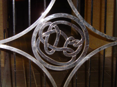
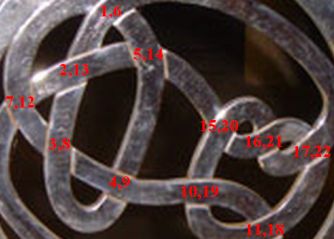
On July 6, 2006, [[User:AnonMoos]] [[User_talk:Drorbn#Here.27s_one|asked]] [[User:Drorbn]] if he could identify the knot in the left hand side picture below. At the time it was impossible using the tools available with <code>KnotTheory`</code> - using any of many invariants, the answer can be found to be either the mirror of [[K11n34]] or the mirror of [[K11n42]], but <code>KnotTheory`</code> couldn't tell which one it is (though of course, it is possible to do it "by hand"). The 2007 addition <math>\widehat{\operatorname{HFK}}</math> does the job, though. Indeed, we first extract the mystery knot's [[DT (Dowker-Thistlethwaite) Codes|DT (Dowker-Thistlethwaite) Code]] using the picture on the right hand side below, then compute <math>\widehat{\operatorname{HFK}}</math>, and then search for it within the <math>\widehat{\operatorname{HFK}}</math>'s of all knots with up to 11 crossings: |
|||
{| align=center width=80% |
|||
|align=center|[[Image:Gateknot.jpg|240px]] |
|||
|align=center|[[Image:Gateknot DT Labeled.png|252px]] |
|||
|} |
|||
<!--$$K3 = DTCode[6, 8, 14, 12, 4, -18, 2, -20, -22, -10, -16];$$--> |
|||
<!--Robot Land, no human edits to "END"--> |
|||
{{In| |
|||
n = 9 | |
|||
in = <nowiki>K3 = DTCode[6, 8, 14, 12, 4, -18, 2, -20, -22, -10, -16];</nowiki>}} |
|||
<!--END--> |
|||
<!--$HFKHat[Mirror[K3]] = Function @@ {3 + 2/m + 1/(m^4 t^3) + 1/(m^3 t^3) + 3/(m^3 t^2) + 3/(m^2 t^2) + 3/(m^2 t) + 3/(m t) + 3 t + 3 m t + 3 m t^2 + 3 m^2 t^2 + m^2 t^3 + m^3 t^3 /. {t -> #1, m -> #2}};$--><!--END--> |
|||
<!--$$H = HFKHat[Mirror[K3]][t, m]$$--> |
|||
<!--Robot Land, no human edits to "END"--> |
|||
{{InOut| |
|||
n = 10 | |
|||
in = <nowiki>H = HFKHat[Mirror[K3]][t, m]</nowiki> | |
|||
out= <nowiki> 2 1 1 3 3 3 3 |
|||
3 + - + ----- + ----- + ----- + ----- + ---- + --- + 3 t + 3 m t + |
|||
m 4 3 3 3 3 2 2 2 2 m t |
|||
m t m t m t m t m t |
|||
2 2 2 2 3 3 3 |
|||
3 m t + 3 m t + m t + m t</nowiki>}} |
|||
<!--END--> |
|||
<!--$$Select[AllKnots[], HFKHat[#][t, m] == H &]$$--> |
|||
<!--Robot Land, no human edits to "END"--> |
|||
{{InOut| |
|||
n = 11 | |
|||
in = <nowiki>Select[AllKnots[], HFKHat[#][t, m] == H &]</nowiki> | |
|||
out= <nowiki>{Knot[11, NonAlternating, 34]}</nowiki>}} |
|||
<!--END--> |
|||
And so the mystery knot is the Conway knot, the mirror of [[K11n34]]. |
|||
Latest revision as of 10:40, 20 March 2008
In 2007, Jean-Marie Droz of the University of Zurich (working along with Anna Beliakova) wrote a Python program to compute the (hat-version) Heegaard-Floer Knot Homology [math]\displaystyle{ \widehat{\operatorname{HFK}}(K) }[/math] of a knot [math]\displaystyle{ K }[/math] (see arXiv:0803.2379). His program is integrated into KnotTheory`, though to run it, you must have Python as well as the Python library Psyco installed on your system.
(For In[1] see Setup)
|
| ||||||||
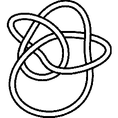
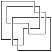
The Heegaard-Floer Knot Homology is a categorification of the Alexander polynomial. Let us test that for the knot 8_19:
In[3]:=
|
hfk = HFKHat[K = Knot[8, 19]][t, m]
|
Out[3]=
|
 2    -3   m     5  2    6  3
m  + t   + -- + m  t  + m  t
            2
           t
|
In[4]:=
|
{hfk /. m -> -1, Alexander[K][t]}
|
Out[4]=
|
      -3    -2    2    3       -3    -2    2    3
{1 + t   - t   - t  + t , 1 + t   - t   - t  + t }
|
The knot 8_19 is the first knot in the Rolfsen Knot Table whose Heegaard-Floer Knot Homology is not "diagonal". Let us test that. The homology [math]\displaystyle{ \widehat{\operatorname{HFK}}(K) }[/math] is "on diagonal", iff its Poincare polynomial, evaluated at [math]\displaystyle{ m=1/t }[/math], is a monomial:
In[5]:=
|
Select[AllKnots[{3, 8}], (Head[HFKHat[#][t, 1/t]] == Plus) &]
|
Out[5]=
|
{Knot[8, 19]}
|
In[6]:=
|
hfk /. m -> 1/t
|
Out[6]=
|
4     -2
-- + t
 3
t
|
 K11n34 |
 K11n42 |
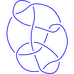
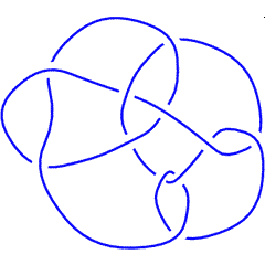
The (mirrored) Conway knot K11n34 and the (mirrored) Kinoshita-Terasaka knot K11n42 are a mutant pair, and are notoriously difficult to tell apart. Let us check that an array of standard knot polynomials fails to separate them, yet [math]\displaystyle{ \widehat{\operatorname{HFK}} }[/math] succeeds:
In[7]:=
|
K1 = Knot["K11n34"]; K2 = Knot["K11n42"];
test[invt_] := (invt[K1] =!= invt[K2]);
test /@ {
  Alexander, MultivariableAlexander, Jones,  HOMFLYPT, Kauffman, Kh, HFKHat
}
|
Out[7]=
|
{False, False, False, False, False, False, True}
|
Indeed,
In[8]:=
|
{HFKHat[K1][t, m], HFKHat[K2][t, m]}
|
Out[8]=
|
     2     1       1       3       3      3      3
{3 + - + ----- + ----- + ----- + ----- + ---- + --- + 3 t + 3 m t +
     m    4  3    3  3    3  2    2  2    2     m t
         m  t    m  t    m  t    m  t    m  t

        2      2  2    2  3    3  3
   3 m t  + 3 m  t  + m  t  + m  t ,

      6     1       1      4      4                     2    2  2
  7 + - + ----- + ----- + ---- + --- + 4 t + 4 m t + m t  + m  t }
      m    3  2    2  2    2     m t
          m  t    m  t    m  t
|
On July 6, 2006, User:AnonMoos asked User:Drorbn if he could identify the knot in the left hand side picture below. At the time it was impossible using the tools available with KnotTheory` - using any of many invariants, the answer can be found to be either the mirror of K11n34 or the mirror of K11n42, but KnotTheory` couldn't tell which one it is (though of course, it is possible to do it "by hand"). The 2007 addition [math]\displaystyle{ \widehat{\operatorname{HFK}} }[/math] does the job, though. Indeed, we first extract the mystery knot's DT (Dowker-Thistlethwaite) Code using the picture on the right hand side below, then compute [math]\displaystyle{ \widehat{\operatorname{HFK}} }[/math], and then search for it within the [math]\displaystyle{ \widehat{\operatorname{HFK}} }[/math]'s of all knots with up to 11 crossings:
|
|
In[9]:=
|
K3 = DTCode[6, 8, 14, 12, 4, -18, 2, -20, -22, -10, -16];
|
In[10]:=
|
H = HFKHat[Mirror[K3]][t, m]
|
Out[10]=
|
    2     1       1       3       3      3      3
3 + - + ----- + ----- + ----- + ----- + ---- + --- + 3 t + 3 m t +
    m    4  3    3  3    3  2    2  2    2     m t
        m  t    m  t    m  t    m  t    m  t

       2      2  2    2  3    3  3
  3 m t  + 3 m  t  + m  t  + m  t
|
In[11]:=
|
Select[AllKnots[], HFKHat[#][t, m] == H &]
|
Out[11]=
|
{Knot[11, NonAlternating, 34]}
|
And so the mystery knot is the Conway knot, the mirror of K11n34.
