10 140

10_139

10_141

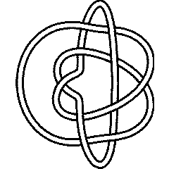
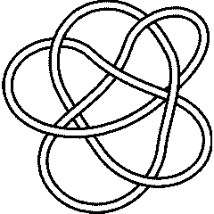
(KnotPlot image)	See the full Rolfsen Knot Table. Visit 10 140's page at the Knot Server (KnotPlot driven, includes 3D interactive images!) Visit 10 140 at Knotilus!
	10_140 is also known as the pretzel knot P(4,3,-3).

Knot presentations

Planar diagram presentation	X1425 X3,10,4,11 X11,19,12,18 X14,5,15,6 X6,17,7,18 X16,7,17,8 X8,15,9,16 X13,1,14,20 X19,13,20,12 X9,2,10,3
Gauss code	-1, 10, -2, 1, 4, -5, 6, -7, -10, 2, -3, 9, -8, -4, 7, -6, 5, 3, -9, 8
Dowker-Thistlethwaite code	4 10 -14 -16 2 18 20 -8 -6 12
Conway Notation	[4,3,21-]

Minimum Braid Representative	A Morse Link Presentation	An Arc Presentation
Length is 11, width is 4, Braid index is 4		[{9, 2}, {1, 7}, {6, 8}, {7, 9}, {10, 13}, {8, 12}, {13, 11}, {12, 5}, {4, 6}, {5, 3}, {2, 4}, {3, 10}, {11, 1}]

[edit Notes on presentations of 10 140]

Computer Talk

The above data is available with the Mathematica package KnotTheory`. Your input (in red) is realistic; all else should have the same content as in a real mathematica session, but with different formatting.

(The path below may be different on your system, and possibly also the KnotTheory` date)

In[1]:=

AppendTo[$Path, "C:/drorbn/projects/KAtlas/"]; << KnotTheory`

Loading KnotTheory` version of May 31, 2006, 14:15:20.091. Read more at http://katlas.org/wiki/KnotTheory.

In[3]:=

K = Knot["10 140"];

In[4]:=

PD[K]

KnotTheory::loading: Loading precomputed data in PD4Knots`.

Out[4]=

X1425 X3,10,4,11 X11,19,12,18 X14,5,15,6 X6,17,7,18 X16,7,17,8 X8,15,9,16 X13,1,14,20 X19,13,20,12 X9,2,10,3

In[5]:=

GaussCode[K]

Out[5]=

-1, 10, -2, 1, 4, -5, 6, -7, -10, 2, -3, 9, -8, -4, 7, -6, 5, 3, -9, 8

In[6]:=

DTCode[K]

Out[6]=

4 10 -14 -16 2 18 20 -8 -6 12

(The path below may be different on your system)

In[7]:=

AppendTo[$Path, "C:/bin/LinKnot/"];

In[8]:=

ConwayNotation[K]

Out[8]=

[4,3,21-]

In[9]:=

br = BR[K]

KnotTheory::credits: The minimum braids representing the knots with up to 10 crossings were provided by Thomas Gittings. See arXiv:math.GT/0401051.

Out[9]=

[math]\displaystyle{ \textrm{BR}(4,\{1,1,1,-2,-1,-1,-1,-2,-3,2,-3\}) }[/math]

In[10]:=

{First[br], Crossings[br], BraidIndex[K]}

KnotTheory::credits: The braid index data known to KnotTheory` is taken from Charles Livingston's http://www.indiana.edu/~knotinfo/.

KnotTheory::loading: Loading precomputed data in IndianaData`.

Out[10]=

{ 4, 11, 4 }

In[11]:=

Show[BraidPlot[br]]

Out[11]=

-Graphics-

In[12]:=

Show[DrawMorseLink[K]]

KnotTheory::credits: "MorseLink was added to KnotTheory` by Siddarth Sankaran at the University of Toronto in the summer of 2005."

KnotTheory::credits: "DrawMorseLink was written by Siddarth Sankaran at the University of Toronto in the summer of 2005."

Out[12]=

-Graphics-

In[13]:=

ap = ArcPresentation[K]

Out[13]=

ArcPresentation[{9, 2}, {1, 7}, {6, 8}, {7, 9}, {10, 13}, {8, 12}, {13, 11}, {12, 5}, {4, 6}, {5, 3}, {2, 4}, {3, 10}, {11, 1}]

In[14]:=

Draw[ap]

Out[14]=

-Graphics-

Three dimensional invariants

Symmetry type Reversible Unknotting number 2 3-genus 2 Bridge index 3 Super bridge index Missing Nakanishi index 2 Maximal Thurston-Bennequin number [-8][-1] Hyperbolic Volume 5.21257 A-Polynomial See Data:10 140/A-polynomial

[edit Notes for 10 140's three dimensional invariants]

Four dimensional invariants

Smooth 4 genus [math]\displaystyle{ 0 }[/math] Topological 4 genus [math]\displaystyle{ 0 }[/math] Concordance genus [math]\displaystyle{ 0 }[/math] Rasmussen s-Invariant 0

[edit Notes for 10 140's four dimensional invariants]

Polynomial invariants

Alexander polynomial	[math]\displaystyle{ t^2-2 t+3-2 t^{-1} + t^{-2} }[/math]
Conway polynomial	[math]\displaystyle{ z^4+2 z^2+1 }[/math]
2nd Alexander ideal (db, data sources)	[math]\displaystyle{ \left\{2,t^2+t+1\right\} }[/math]
Determinant and Signature	{ 9, 0 }
Jones polynomial	[math]\displaystyle{ 1- q^{-1} + q^{-2} - q^{-3} +2 q^{-4} - q^{-5} + q^{-6} - q^{-7} }[/math]
HOMFLY-PT polynomial (db, data sources)	[math]\displaystyle{ -z^2 a^6-2 a^6+z^4 a^4+4 z^2 a^4+4 a^4-z^2 a^2-2 a^2+1 }[/math]
Kauffman polynomial (db, data sources)	[math]\displaystyle{ a^6 z^8+a^4 z^8+a^7 z^7+2 a^5 z^7+a^3 z^7-6 a^6 z^6-6 a^4 z^6-6 a^7 z^5-11 a^5 z^5-5 a^3 z^5+11 a^6 z^4+12 a^4 z^4+a^2 z^4+10 a^7 z^3+16 a^5 z^3+6 a^3 z^3-8 a^6 z^2-12 a^4 z^2-4 a^2 z^2-4 a^7 z-6 a^5 z-2 a^3 z+2 a^6+4 a^4+2 a^2+1 }[/math]
The A2 invariant	[math]\displaystyle{ -q^{22}-q^{20}-q^{18}+2 q^{14}+2 q^{12}+2 q^{10}-q^6-q^4+1+ q^{-2} }[/math]
The G2 invariant	[math]\displaystyle{ q^{108}+q^{104}-q^{102}-q^{96}+q^{94}-q^{92}-q^{90}-q^{88}-q^{86}-q^{82}-4 q^{80}-4 q^{70}+q^{68}+3 q^{66}-q^{62}-q^{60}+3 q^{58}+5 q^{56}+2 q^{54}-q^{52}+q^{50}+3 q^{48}+4 q^{46}-2 q^{42}+q^{40}+3 q^{38}+q^{36}-q^{34}-2 q^{30}+q^{28}-3 q^{24}-q^{20}-q^{18}+q^{16}-q^{14}-q^{12}-q^8+q^6+2+ q^{-4} + q^{-6} + q^{-10} }[/math]

Further Quantum Invariants

Further quantum knot invariants for 10_140.

A1 Invariants.

Weight	Invariant
1	[math]\displaystyle{ -q^{15}+q^9+q^7+ q^{-1} }[/math]
2	[math]\displaystyle{ q^{44}-q^{40}-q^{34}-q^{32}+q^{28}+q^{26}+q^{22}-q^{18}-q^{14}-q^{12}+q^{10}+q^8+q^6+q^2+2- q^{-4} }[/math]
3	[math]\displaystyle{ -q^{87}+q^{83}+q^{81}-q^{77}+q^{73}+q^{71}-q^{67}-2 q^{65}-q^{63}+q^{59}-q^{55}+2 q^{51}+2 q^{49}-q^{45}+q^{41}-2 q^{37}-2 q^{35}-q^{29}+q^{25}+q^{23}+q^{17}+q^{15}-q^{11}-q^9+2 q^7+3 q^5-2 q+3 q^{-3} + q^{-5} - q^{-7} - q^{-9} }[/math]

A2 Invariants.

Weight	Invariant
1,0	[math]\displaystyle{ -q^{22}-q^{20}-q^{18}+2 q^{14}+2 q^{12}+2 q^{10}-q^6-q^4+1+ q^{-2} }[/math]
1,1	[math]\displaystyle{ q^{60}+2 q^{56}-2 q^{54}+2 q^{52}-2 q^{50}-2 q^{46}-4 q^{44}-4 q^{40}+2 q^{38}+q^{36}+4 q^{34}+4 q^{32}+4 q^{30}+q^{28}-2 q^{26}-4 q^{24}-4 q^{22}-4 q^{20}-2 q^{18}+6 q^{14}+2 q^{12}+6 q^{10}+2 q^8+2 q^4-2 q^2+2-2 q^{-2} + q^{-4} }[/math]
2,0	[math]\displaystyle{ q^{58}+q^{56}+q^{54}-q^{48}-2 q^{46}-4 q^{44}-4 q^{42}-3 q^{40}+4 q^{36}+4 q^{34}+6 q^{32}+4 q^{30}+3 q^{28}-2 q^{26}-4 q^{24}-5 q^{22}-5 q^{20}-3 q^{18}+4 q^{14}+4 q^{12}+5 q^{10}+2 q^8+1- q^{-2} }[/math]

A3 Invariants.

Weight	Invariant
0,1,0	[math]\displaystyle{ q^{46}+q^{42}-q^{38}-2 q^{36}-2 q^{34}-2 q^{32}-3 q^{30}+2 q^{24}+2 q^{22}+4 q^{20}+3 q^{18}+2 q^{16}+2 q^{14}-q^{10}-2 q^8-q^6-q^4+2+ q^{-2} + q^{-4} }[/math]
1,0,0	[math]\displaystyle{ -q^{29}-q^{27}-2 q^{25}-q^{23}+2 q^{19}+3 q^{17}+3 q^{15}+2 q^{13}-q^9-2 q^7-q^5+q+ q^{-1} + q^{-3} }[/math]

A4 Invariants.

Weight	Invariant
0,1,0,0	[math]\displaystyle{ q^{60}+q^{58}+2 q^{56}+2 q^{54}+q^{52}-q^{50}-3 q^{48}-6 q^{46}-7 q^{44}-6 q^{42}-4 q^{40}-q^{38}+2 q^{36}+6 q^{34}+6 q^{32}+5 q^{30}+4 q^{28}+3 q^{26}+q^{22}+q^{20}+q^{18}+q^{16}+q^{14}-2 q^{10}-2 q^8-q^6-q^4+2+2 q^{-2} + q^{-4} + q^{-6} }[/math]
1,0,0,0	[math]\displaystyle{ -q^{36}-q^{34}-2 q^{32}-2 q^{30}-q^{28}+2 q^{24}+3 q^{22}+4 q^{20}+3 q^{18}+2 q^{16}-q^{12}-2 q^{10}-2 q^8-q^6+q^2+1+ q^{-2} + q^{-4} }[/math]

B2 Invariants.

Weight	Invariant
0,1	[math]\displaystyle{ -q^{46}-q^{42}-q^{38}+q^{30}+2 q^{26}+2 q^{22}+q^{18}-q^{10}-q^6+q^4+ q^{-2} + q^{-4} }[/math]
1,0	[math]\displaystyle{ q^{76}+q^{68}-q^{64}-q^{62}-q^{58}-2 q^{56}-q^{54}-q^{48}+q^{42}+q^{38}+q^{34}+q^{32}+q^{30}+q^{26}+2 q^{24}+q^{22}+q^{16}-q^{12}-q^{10}-q^4+1+ q^{-2} + q^{-6} }[/math]

D4 Invariants.

Weight	Invariant
1,0,0,0	[math]\displaystyle{ q^{62}+q^{58}+q^{54}-q^{52}-q^{50}-2 q^{48}-3 q^{46}-3 q^{44}-4 q^{42}-2 q^{40}-2 q^{38}+q^{36}+q^{34}+4 q^{32}+4 q^{30}+6 q^{28}+4 q^{26}+4 q^{24}+2 q^{22}+q^{20}-2 q^{16}-2 q^{14}-3 q^{12}-q^{10}-2 q^8+q^2+2+ q^{-2} + q^{-4} + q^{-6} }[/math]

G2 Invariants.

Weight	Invariant
1,0	[math]\displaystyle{ q^{108}+q^{104}-q^{102}-q^{96}+q^{94}-q^{92}-q^{90}-q^{88}-q^{86}-q^{82}-4 q^{80}-4 q^{70}+q^{68}+3 q^{66}-q^{62}-q^{60}+3 q^{58}+5 q^{56}+2 q^{54}-q^{52}+q^{50}+3 q^{48}+4 q^{46}-2 q^{42}+q^{40}+3 q^{38}+q^{36}-q^{34}-2 q^{30}+q^{28}-3 q^{24}-q^{20}-q^{18}+q^{16}-q^{14}-q^{12}-q^8+q^6+2+ q^{-4} + q^{-6} + q^{-10} }[/math]

.

Computer Talk

The above data is available with the Mathematica package KnotTheory`, as shown in the (simulated) Mathematica session below. Your input (in red) is realistic; all else should have the same content as in a real mathematica session, but with different formatting. This Mathematica session is also available (albeit only for the knot 5_2) as the notebook PolynomialInvariantsSession.nb.

(The path below may be different on your system, and possibly also the KnotTheory` date)

In[1]:=

AppendTo[$Path, "C:/drorbn/projects/KAtlas/"]; << KnotTheory`

Loading KnotTheory` version of August 31, 2006, 11:25:27.5625. Read more at http://katlas.math.toronto.edu/wiki/KnotTheory.

In[3]:=

K = Knot["10 140"];

In[4]:=

Alexander[K][t]

KnotTheory::loading: Loading precomputed data in PD4Knots`.

Out[4]=

[math]\displaystyle{ t^2-2 t+3-2 t^{-1} + t^{-2} }[/math]

In[5]:=

Conway[K][z]

Out[5]=

[math]\displaystyle{ z^4+2 z^2+1 }[/math]

In[6]:=

Alexander[K, 2][t]

KnotTheory::credits: The program Alexander[K, r] to compute Alexander ideals was written by Jana Archibald at the University of Toronto in the summer of 2005.

Out[6]=

[math]\displaystyle{ \left\{2,t^2+t+1\right\} }[/math]

In[7]:=

{KnotDet[K], KnotSignature[K]}

Out[7]=

{ 9, 0 }

In[8]:=

Jones[K][q]

KnotTheory::loading: Loading precomputed data in Jones4Knots`.

Out[8]=

[math]\displaystyle{ 1- q^{-1} + q^{-2} - q^{-3} +2 q^{-4} - q^{-5} + q^{-6} - q^{-7} }[/math]

In[9]:=

HOMFLYPT[K][a, z]

KnotTheory::credits: The HOMFLYPT program was written by Scott Morrison.

Out[9]=

[math]\displaystyle{ -z^2 a^6-2 a^6+z^4 a^4+4 z^2 a^4+4 a^4-z^2 a^2-2 a^2+1 }[/math]

In[10]:=

Kauffman[K][a, z]

KnotTheory::loading: Loading precomputed data in Kauffman4Knots`.

Out[10]=

[math]\displaystyle{ a^6 z^8+a^4 z^8+a^7 z^7+2 a^5 z^7+a^3 z^7-6 a^6 z^6-6 a^4 z^6-6 a^7 z^5-11 a^5 z^5-5 a^3 z^5+11 a^6 z^4+12 a^4 z^4+a^2 z^4+10 a^7 z^3+16 a^5 z^3+6 a^3 z^3-8 a^6 z^2-12 a^4 z^2-4 a^2 z^2-4 a^7 z-6 a^5 z-2 a^3 z+2 a^6+4 a^4+2 a^2+1 }[/math]

"Similar" Knots (within the Atlas)

Same Alexander/Conway Polynomial: {8_20, K11n73, K11n74,}

Same Jones Polynomial (up to mirroring, [math]\displaystyle{ q\leftrightarrow q^{-1} }[/math]): {}

Computer Talk

The above data is available with the Mathematica package KnotTheory`. Your input (in red) is realistic; all else should have the same content as in a real mathematica session, but with different formatting.

(The path below may be different on your system, and possibly also the KnotTheory` date)

In[1]:=

AppendTo[$Path, "C:/drorbn/projects/KAtlas/"]; << KnotTheory`

Loading KnotTheory` version of May 31, 2006, 14:15:20.091. Read more at http://katlas.math.toronto.edu/wiki/KnotTheory.

In[3]:=

K = Knot["10 140"];

In[4]:=

{A = Alexander[K][t], J = Jones[K][q]}

KnotTheory::loading: Loading precomputed data in PD4Knots`.

KnotTheory::loading: Loading precomputed data in Jones4Knots`.

Out[4]=

{ [math]\displaystyle{ t^2-2 t+3-2 t^{-1} + t^{-2} }[/math], [math]\displaystyle{ 1- q^{-1} + q^{-2} - q^{-3} +2 q^{-4} - q^{-5} + q^{-6} - q^{-7} }[/math] }

In[5]:=

DeleteCases[Select[AllKnots[], (A === Alexander[#][t]) &], K]

KnotTheory::loading: Loading precomputed data in DTCode4KnotsTo11`.

KnotTheory::credits: The GaussCode to PD conversion was written by Siddarth Sankaran at the University of Toronto in the summer of 2005.

Out[5]=

{8_20, K11n73, K11n74,}

In[6]:=

DeleteCases[ Select[ AllKnots[], (J === Jones[#][q] || (J /. q -> 1/q) === Jones[#][q]) & ], K ]

KnotTheory::loading: Loading precomputed data in Jones4Knots11`.

Out[6]=

{}

Vassiliev invariants

V2 and V3:

(2, -4)

V2,1 through V6,9:

V2,1 V3,1 V4,1 V4,2 V4,3 V5,1 V5,2 V5,3 V5,4 V6,1 V6,2 V6,3 V6,4 V6,5 V6,6 V6,7 V6,8 V6,9 [math]\displaystyle{ 8 }[/math] [math]\displaystyle{ -32 }[/math] [math]\displaystyle{ 32 }[/math] [math]\displaystyle{ \frac{316}{3} }[/math] [math]\displaystyle{ \frac{20}{3} }[/math] [math]\displaystyle{ -256 }[/math] [math]\displaystyle{ -\frac{1472}{3} }[/math] [math]\displaystyle{ -\frac{128}{3} }[/math] [math]\displaystyle{ -96 }[/math] [math]\displaystyle{ \frac{256}{3} }[/math] [math]\displaystyle{ 512 }[/math] [math]\displaystyle{ \frac{2528}{3} }[/math] [math]\displaystyle{ \frac{160}{3} }[/math] [math]\displaystyle{ \frac{33391}{15} }[/math] [math]\displaystyle{ -\frac{2444}{15} }[/math] [math]\displaystyle{ \frac{43564}{45} }[/math] [math]\displaystyle{ \frac{881}{9} }[/math] [math]\displaystyle{ \frac{1711}{15} }[/math]

V_2,1 through V_6,9 were provided by Petr Dunin-Barkowski <barkovs@itep.ru>, Andrey Smirnov <asmirnov@itep.ru>, and Alexei Sleptsov <sleptsov@itep.ru> and uploaded on October 2010 by User:Drorbn. Note that they are normalized differently than V₂ and V₃.

Khovanov Homology

The coefficients of the monomials [math]\displaystyle{ t^rq^j }[/math] are shown, along with their alternating sums [math]\displaystyle{ \chi }[/math] (fixed [math]\displaystyle{ j }[/math], alternation over [math]\displaystyle{ r }[/math]). The squares with yellow highlighting are those on the "critical diagonals", where [math]\displaystyle{ j-2r=s+1 }[/math] or [math]\displaystyle{ j-2r=s-1 }[/math], where [math]\displaystyle{ s= }[/math]0 is the signature of 10 140. Nonzero entries off the critical diagonals (if any exist) are highlighted in red.

\   r    \    j   \ -7 -6 -5 -4 -3 -2 -1 0 χ 1               1 1 -1             1 1 0 -3                 0 -5         1 1     0 -7       1         1 -9       1         1 -11   1 1           0 -13                 0 -15 1               -1

Integral Khovanov Homology (db, data source)

[math]\displaystyle{ \dim{\mathcal G}_{2r+i}\operatorname{KH}^r_{\mathbb Z} }[/math] [math]\displaystyle{ i=-1 }[/math] [math]\displaystyle{ i=1 }[/math] [math]\displaystyle{ r=-7 }[/math] [math]\displaystyle{ {\mathbb Z} }[/math] [math]\displaystyle{ r=-6 }[/math] [math]\displaystyle{ {\mathbb Z}_2 }[/math] [math]\displaystyle{ {\mathbb Z} }[/math] [math]\displaystyle{ r=-5 }[/math] [math]\displaystyle{ {\mathbb Z} }[/math] [math]\displaystyle{ r=-4 }[/math] [math]\displaystyle{ {\mathbb Z}\oplus{\mathbb Z}_2 }[/math] [math]\displaystyle{ {\mathbb Z} }[/math] [math]\displaystyle{ r=-3 }[/math] [math]\displaystyle{ {\mathbb Z}_2 }[/math] [math]\displaystyle{ {\mathbb Z} }[/math] [math]\displaystyle{ r=-2 }[/math] [math]\displaystyle{ {\mathbb Z} }[/math] [math]\displaystyle{ r=-1 }[/math] [math]\displaystyle{ {\mathbb Z}_2 }[/math] [math]\displaystyle{ {\mathbb Z} }[/math] [math]\displaystyle{ r=0 }[/math] [math]\displaystyle{ {\mathbb Z} }[/math] [math]\displaystyle{ {\mathbb Z} }[/math]

The Coloured Jones Polynomials

The Coloured Jones Polynomials (in the [math]\displaystyle{ n+1 }[/math]-dimensional representation of [math]\displaystyle{ sl(2) }[/math])

[math]\displaystyle{ n }[/math]	[math]\displaystyle{ J_n }[/math]
2	[math]\displaystyle{ -q+1+2 q^{-1} -2 q^{-2} +3 q^{-4} -2 q^{-5} + q^{-7} -2 q^{-8} + q^{-9} - q^{-11} +2 q^{-12} - q^{-13} +2 q^{-15} -2 q^{-16} - q^{-17} +2 q^{-18} - q^{-19} - q^{-20} + q^{-21} }[/math]
3	[math]\displaystyle{ -q^3+2 q+2-4 q^{-1} -2 q^{-2} +4 q^{-3} +5 q^{-4} -5 q^{-5} -5 q^{-6} +4 q^{-7} +6 q^{-8} -4 q^{-9} -5 q^{-10} +3 q^{-11} +6 q^{-12} -3 q^{-13} -5 q^{-14} +2 q^{-15} +5 q^{-16} -2 q^{-17} -5 q^{-18} +5 q^{-20} -4 q^{-22} - q^{-23} +4 q^{-24} + q^{-25} -2 q^{-26} - q^{-27} +2 q^{-28} - q^{-30} + q^{-32} - q^{-33} -2 q^{-34} + q^{-35} +2 q^{-36} -2 q^{-38} + q^{-40} + q^{-41} - q^{-42} }[/math]
4	[math]\displaystyle{ q^3-2 q^2-2 q+4 q^{-1} +7 q^{-2} -5 q^{-3} -6 q^{-4} -4 q^{-5} +6 q^{-6} +12 q^{-7} -4 q^{-8} -7 q^{-9} -8 q^{-10} +4 q^{-11} +14 q^{-12} -3 q^{-13} -6 q^{-14} -7 q^{-15} +3 q^{-16} +11 q^{-17} -4 q^{-18} -4 q^{-19} -5 q^{-20} +3 q^{-21} +9 q^{-22} -3 q^{-23} -2 q^{-24} -5 q^{-25} + q^{-26} +7 q^{-27} - q^{-28} -5 q^{-30} -2 q^{-31} +4 q^{-32} +3 q^{-34} -2 q^{-35} -4 q^{-36} +5 q^{-39} +2 q^{-40} -3 q^{-41} -3 q^{-42} -2 q^{-43} +3 q^{-44} +5 q^{-45} -3 q^{-47} -3 q^{-48} - q^{-49} +4 q^{-50} - q^{-53} -2 q^{-54} +3 q^{-55} -2 q^{-56} +4 q^{-60} -2 q^{-61} - q^{-62} - q^{-63} - q^{-64} +3 q^{-65} - q^{-68} - q^{-69} + q^{-70} }[/math]

Computer Talk

Much of the above data can be recomputed by Mathematica using the package KnotTheory`. See A Sample KnotTheory` Session, or any of the Computer Talk sections above.

Modifying This Page

Read me first: Modifying Knot Pages See/edit the Rolfsen Knot Page master template (intermediate). See/edit the Rolfsen_Splice_Base (expert). Back to the top.

10_139 10_141