Three Dimensional Invariants: Difference between revisions
DrorsRobot (talk | contribs) No edit summary |
|||
| (33 intermediate revisions by 7 users not shown) | |||
| Line 2: | Line 2: | ||
{{Startup Note}} |
{{Startup Note}} |
||
====Symmetry Type==== |
|||
<!--$$?SymmetryType$$--> |
<!--$$?SymmetryType$$--> |
||
<!--Robot Land, no human edits to "END"--> |
|||
<!--The lines to END were generated by WikiSplice: do not edit; see manual.--> |
|||
{{HelpAndAbout| |
|||
{{HelpAndAbout1|n=2|s=SymmetryType}} |
|||
n = 2 | |
|||
SymmetryType[K] returns the symmetry type of the knot K, if known to KnotTheory`. The possible types are: Reversible, FullyAmphicheiral, NegativeAmphicheiral and Chiral. |
|||
n1 = 3 | |
|||
{{HelpAndAbout2|n=3|s=SymmetryType}} |
|||
in = <nowiki>SymmetryType</nowiki> | |
|||
The symmetry type data known to KnotTheory` is taken from Charles Livingston's "Table of Knot Invariants", http://www.indiana.edu/~knotinfo/. |
|||
out= <nowiki>SymmetryType[K] returns the symmetry type of the knot K, if known to KnotTheory`. The possible types are: Reversible, FullyAmphicheiral, NegativeAmphicheiral and Chiral.</nowiki> | |
|||
{{HelpAndAbout3}} |
|||
about= <nowiki>The symmetry type data known to KnotTheory` is taken from Charles Livingston's "Table of Knot Invariants", http://www.indiana.edu/~knotinfo/.</nowiki>}} |
|||
<!--END--> |
<!--END--> |
||
The inverse of a knot <math>K</math> is the knot obtained from it by reversing its parametrization. The mirror of A knot <math>K</math> is obtained from <math>K</math> by reversing the orientation of the ambient space, or, alternatively, by flipping all the crossings of <math>K</math>. |
|||
A knot is called "fully amphicheiral" if it is equal to its inverse and also to its mirror. The first knot with this property is |
|||
<!--$$Select[AllKnots[], |
|||
(SymmetryType[#] == FullyAmphicheiral) &, 1]$$--> |
|||
<!--Robot Land, no human edits to "END"--> |
|||
{{InOut| |
|||
n = 4 | |
|||
in = <nowiki>Select[AllKnots[], |
|||
(SymmetryType[#] == FullyAmphicheiral) &, 1]</nowiki> | |
|||
out= <nowiki>{Knot[4, 1]}</nowiki>}} |
|||
<!--END--> |
|||
A knot is called "reversible" if it is equal to its inverse yet it different from its mirror (and hence also from the inverse of its mirror). Many knots have this property; indeed, the first one is: |
|||
<!--$$Select[AllKnots[], |
|||
(SymmetryType[#] == Reversible) &, 1]$$--> |
|||
<!--Robot Land, no human edits to "END"--> |
|||
{{InOut| |
|||
n = 5 | |
|||
in = <nowiki>Select[AllKnots[], |
|||
(SymmetryType[#] == Reversible) &, 1]</nowiki> | |
|||
out= <nowiki>{Knot[3, 1]}</nowiki>}} |
|||
<!--END--> |
|||
A knot is called "positive amphicheiral" if it is different from its inverse but equal to its mirror. There are no such knots with up to 11 crossings. |
|||
A knot is called "negative amphicheiral" if it is different from its inverse and its mirror, yet it is equal to the inverse of its mirror. The first knot with this property is |
|||
<!--$$Select[AllKnots[], |
|||
(SymmetryType[#] == NegativeAmphicheiral) &, 1]$$--> |
|||
<!--Robot Land, no human edits to "END"--> |
|||
{{InOut| |
|||
n = 6 | |
|||
in = <nowiki>Select[AllKnots[], |
|||
(SymmetryType[#] == NegativeAmphicheiral) &, 1]</nowiki> | |
|||
out= <nowiki>{Knot[8, 17]}</nowiki>}} |
|||
<!--END--> |
|||
Finally, if a knot is different from its inverse, its mirror and from the inverse of its mirror, it is "chiral". The first such knot is |
|||
<!--$$Select[AllKnots[], |
|||
(SymmetryType[#] == Chiral) &, 1]$$--> |
|||
<!--Robot Land, no human edits to "END"--> |
|||
{{InOut| |
|||
n = 7 | |
|||
in = <nowiki>Select[AllKnots[], |
|||
(SymmetryType[#] == Chiral) &, 1]</nowiki> | |
|||
out= <nowiki>{Knot[9, 32]}</nowiki>}} |
|||
<!--END--> |
|||
It is a amusing to take "symmetry type" statistics on all the prime knots with up to 11 crossings: |
|||
<!--$$Plus @@ (SymmetryType /@ Rest[AllKnots[]])$$--> |
|||
<!--Robot Land, no human edits to "END"--> |
|||
{{InOut| |
|||
n = 8 | |
|||
in = <nowiki>Plus @@ (SymmetryType /@ Rest[AllKnots[]])</nowiki> | |
|||
out= <nowiki>216 Chiral + 13 FullyAmphicheiral + 7 NegativeAmphicheiral + |
|||
565 Reversible</nowiki>}} |
|||
<!--END--> |
|||
{{Knot Image Quadruple|4_1|gif|3_1|gif|8_17|gif|9_32|gif}} |
|||
====Unknotting Number==== |
|||
The ''unknotting number'' of a knot <math>K</math> is the minimal number of crossing changes needed in order to unknot <math>K</math>. |
The ''unknotting number'' of a knot <math>K</math> is the minimal number of crossing changes needed in order to unknot <math>K</math>. |
||
<!--$$?UnknottingNumber$$--> |
<!--$$?UnknottingNumber$$--> |
||
<!--Robot Land, no human edits to "END"--> |
|||
<!--The lines to END were generated by WikiSplice: do not edit; see manual.--> |
|||
{{HelpAndAbout| |
|||
{{HelpAndAbout1|n=4|s=UnknottingNumber}} |
|||
n = 9 | |
|||
UnknottingNumber[K] returns the unknotting number of the knot K, if known to KnotTheory`. If only a range of possible values is known, a list of the form {min, max} is returned. |
|||
n1 = 10 | |
|||
{{HelpAndAbout2|n=5|s=UnknottingNumber}} |
|||
in = <nowiki>UnknottingNumber</nowiki> | |
|||
The unknotting numbers of torus knots are due to ???. All other unknotting numbers known to KnotTheory` are taken from Charles Livingston's "Table of Knot Invariants", http://www.indiana.edu/~knotinfo/. |
|||
out= <nowiki>UnknottingNumber[K] returns the unknotting number of the knot K, if known to KnotTheory`. If only a range of possible values is known, a list of the form {min, max} is returned.</nowiki> | |
|||
{{HelpAndAbout3}} |
|||
about= <nowiki>The unknotting numbers of torus knots are due to ???. All other unknotting numbers known to KnotTheory` are taken from Charles Livingston's "Table of Knot Invariants", http://www.indiana.edu/~knotinfo/.</nowiki>}} |
|||
<!--END--> |
<!--END--> |
||
<!--$UH = Plus @@ u /@ Cases[UnknottingNumber /@ AllKnots[], _Integer];$--><!--END--> |
<!--$UH = Plus @@ u /@ Cases[UnknottingNumber /@ AllKnots[], _Integer];$--><!--END--> |
||
Of the <!--$UH /. _u -> 1$--><!-- |
Of the <!--$UH /. _u -> 1$--><!--Robot Land, no human edits to "END"-->512<!--END--> knots whose unknotting number is known to <code>KnotTheory`</code>, <!--$Coefficient[UH, u[1]]$--><!--Robot Land, no human edits to "END"-->197<!--END--> have unknotting number 1, <!--$Coefficient[UH, u[2]]$--><!--Robot Land, no human edits to "END"-->247<!--END--> have unknotting number 2, <!--$Coefficient[UH, u[3]]$--><!--Robot Land, no human edits to "END"-->54<!--END--> have unknotting number 3, <!--$Coefficient[UH, u[4]]$--><!--Robot Land, no human edits to "END"-->12<!--END--> have unknotting number 4 and <!--$Coefficient[UH, u[5]]$--><!--Robot Land, no human edits to "END"-->1<!--END--> has unknotting number 5: |
||
<!--$$Plus @@ u /@ Cases[UnknottingNumber /@ AllKnots[], _Integer]$$--> |
<!--$$Plus @@ u /@ Cases[UnknottingNumber /@ AllKnots[], _Integer]$$--> |
||
<!--Robot Land, no human edits to "END"--> |
|||
<!--The lines to END were generated by WikiSplice: do not edit; see manual.--> |
|||
{{ |
{{InOut| |
||
n = 11 | |
|||
Plus @@ u /@ Cases[UnknottingNumber /@ AllKnots[], _Integer] |
|||
in = <nowiki>Plus @@ u /@ Cases[UnknottingNumber /@ AllKnots[], _Integer]</nowiki> | |
|||
out= <nowiki>u[0] + 197 u[1] + 247 u[2] + 54 u[3] + 12 u[4] + u[5]</nowiki>}} |
|||
{{InOut3}} |
|||
<!--END--> |
<!--END--> |
||
There are <!--$Length[Select[AllKnots[], Crossings[#] <= 9 && Head[UnknottingNumber[#]] === List &] |
There are <!--$Length[Select[AllKnots[], Crossings[#] <= 9 && Head[UnknottingNumber[#]] === List &] |
||
]$--><!-- |
]$--><!--Robot Land, no human edits to "END"-->4<!--END--> knots with up to 9 crossings whose unknotting number is unknown: |
||
<!--$$Select[AllKnots[], |
<!--$$Select[AllKnots[], |
||
Crossings[#] <= 9 && Head[UnknottingNumber[#]] === List & |
|||
<!--The lines to END were generated by WikiSplice: do not edit; see manual.--> |
|||
]$$--> |
|||
{{InOut1|n=7}} |
|||
<!--Robot Land, no human edits to "END"--> |
|||
Select[AllKnots[], Crossings[#] <= 9 && Head[UnknottingNumber[#]] === List &] |
|||
{{InOut| |
|||
{{InOut2|n=7}}<pre style="border: 0px; padding: 0em"><nowiki>{Knot[9, 10], Knot[9, 13], Knot[9, 35], Knot[9, 38]}</nowiki></pre> |
|||
n = 12 | |
|||
{{InOut3}} |
|||
in = <nowiki>Select[AllKnots[], |
|||
Crossings[#] <= 9 && Head[UnknottingNumber[#]] === List & |
|||
]</nowiki> | |
|||
out= <nowiki>{Knot[9, 10], Knot[9, 13], Knot[9, 35], Knot[9, 38]}</nowiki>}} |
|||
<!--END--> |
<!--END--> |
||
{{Knot Image Quadruple|9_10|gif|9_13|gif|9_35|gif|9_38|gif}} |
|||
====3-Genus==== |
|||
A Seifert surface for a knot <math>K \subset S^3</math> is a compact oriented surface <math>L \subset S^3</math> |
|||
with boundary <math>\partial L=K</math>. Seifert surfaces exist, but are not unique. The [http://www.win.tue.nl/~vanwijk/seifertview/ SeifertView programme] is a visual implementation of the algorithm of Seifert (1934) for |
|||
the construction of a Seifert surface from a knot projection. The 3-genus of a knot is the minimal genus of a |
|||
Seifert surface for that knot. |
|||
<!--$$?ThreeGenus$$--> |
<!--$$?ThreeGenus$$--> |
||
<!--Robot Land, no human edits to "END"--> |
|||
<!--The lines to END were generated by WikiSplice: do not edit; see manual.--> |
|||
{{HelpAndAbout| |
|||
{{HelpAndAbout1|n=8|s=ThreeGenus}} |
|||
n = 13 | |
|||
ThreeGenus[K] returns the 3-genus of the knot K, if known to KnotTheory`. |
|||
n1 = 14 | |
|||
{{HelpAndAbout2|n=9|s=ThreeGenus}} |
|||
in = <nowiki>ThreeGenus</nowiki> | |
|||
The 3-genus data known to KnotTheory` is taken from Charles Livingston's "Table of Knot Invariants", http://www.indiana.edu/~knotinfo/. |
|||
out= <nowiki>ThreeGenus[K] returns the 3-genus of the knot K or a list of the form {lower bound, upper bound}.</nowiki> | |
|||
{{HelpAndAbout3}} |
|||
about= <nowiki>The 3-genus program was written by Jake Rasmussen of Princeton University. The program tries to compute the highest nonvanishing group in the knot Floer homology, using Ozsvath and Szabo's version of the Kauffman state model.</nowiki>}} |
|||
<!--END--> |
<!--END--> |
||
The highest 3-genus of the knots known to <tt>KnotTheory`</tt> is <math>5</math>, and there is only one knot with up to 11 crossings whose 3-genus is 5: |
|||
<!--$$Max[ThreeGenus /@ AllKnots[]]$$--> |
|||
<!--Robot Land, no human edits to "END"--> |
|||
{{InOut| |
|||
n = 15 | |
|||
in = <nowiki>Max[ThreeGenus /@ AllKnots[]]</nowiki> | |
|||
out= <nowiki>5</nowiki>}} |
|||
<!--END--> |
|||
<!--$$Select[AllKnots[], ThreeGenus[#] == 5 &]$$--> |
|||
<!--Robot Land, no human edits to "END"--> |
|||
{{InOut| |
|||
n = 16 | |
|||
in = <nowiki>Select[AllKnots[], ThreeGenus[#] == 5 &]</nowiki> | |
|||
out= <nowiki>{Knot[11, Alternating, 367]}</nowiki>}} |
|||
<!--END--> |
|||
{{Knot Image Pair|K11a367|gif|T(11,2)|jpg}} |
|||
([[K11a367]] is, of couse, also known as the torus knot [[T(11,2)]]). |
|||
The Conway knot [[K11n34]] is the closure of the braid <tt>BR[4, {1, 1, 2, -3, 2, 1, -3, -2, -2, -3, -3}]</tt>. Let us compute its 3-genus and compare it with the 3-genus of its mutant companion, the Kinoshita-Terasaka knot [[K11n42]]: |
|||
<!--$$ThreeGenus[BR[4, {1, 1, 2, -3, 2, 1, -3, -2, -2, -3, -3}]]$$--> |
|||
<!--Robot Land, no human edits to "END"--> |
|||
{{InOut| |
|||
n = 17 | |
|||
in = <nowiki>ThreeGenus[BR[4, {1, 1, 2, -3, 2, 1, -3, -2, -2, -3, -3}]]</nowiki> | |
|||
out= <nowiki>3</nowiki>}} |
|||
<!--END--> |
|||
<!--$$ThreeGenus[Knot[11, NonAlternating, 42]]$$--> |
|||
<!--Robot Land, no human edits to "END"--> |
|||
{{InOut| |
|||
n = 18 | |
|||
in = <nowiki>ThreeGenus[Knot[11, NonAlternating, 42]]</nowiki> | |
|||
out= <nowiki>2</nowiki>}} |
|||
<!--END--> |
|||
{{Knot Image Pair|K11n34|gif|K11n42|gif}} |
|||
====Bridge Index==== |
|||
The ''bridge index' of a knot <math>K</math> is the minimal number of local maxima (or local minima) in a generic smooth embedding of <math>K</math> in <math>{\mathbf R}^3</math>. |
The ''bridge index' of a knot <math>K</math> is the minimal number of local maxima (or local minima) in a generic smooth embedding of <math>K</math> in <math>{\mathbf R}^3</math>. |
||
<!--$$?BridgeIndex$$--> |
<!--$$?BridgeIndex$$--> |
||
<!--Robot Land, no human edits to "END"--> |
|||
<!--The lines to END were generated by WikiSplice: do not edit; see manual.--> |
|||
{{HelpAndAbout| |
|||
{{HelpAndAbout1|n=10|s=BridgeIndex}} |
|||
n = 19 | |
|||
BridgeIndex[K] returns the bridge index of the knot K, if known to KnotTheory`. |
|||
n1 = 20 | |
|||
{{HelpAndAbout2|n=11|s=BridgeIndex}} |
|||
in = <nowiki>BridgeIndex</nowiki> | |
|||
The bridge index data known to KnotTheory` is taken from Charles Livingston's "Table of Knot Invariants", http://www.indiana.edu/~knotinfo/. |
|||
out= <nowiki>BridgeIndex[K] returns the bridge index of the knot K, if known to KnotTheory`.</nowiki> | |
|||
{{HelpAndAbout3}} |
|||
about= <nowiki>The bridge index data known to KnotTheory` is taken from Charles Livingston's "Table of Knot Invariants", http://www.indiana.edu/~knotinfo/.</nowiki>}} |
|||
<!--END--> |
<!--END--> |
||
An often studied class of knots is the class of 2-bridge knots, knots whose bridge index is 2. Of the 49 9-crossings knots, 24 are 2-bridge: |
An often studied class of knots is the class of 2-bridge knots, knots whose bridge index is 2. Of the 49 prime 9-crossings knots, 24 are 2-bridge: |
||
<!--$$Select[AllKnots[], Crossings[#] == 9 && BridgeIndex[#] == 2 &]$$--> |
<!--$$Select[AllKnots[], Crossings[#] == 9 && BridgeIndex[#] == 2 &]$$--> |
||
<!--Robot Land, no human edits to "END"--> |
|||
<!--The lines to END were generated by WikiSplice: do not edit; see manual.--> |
|||
{{InOut| |
|||
{{InOut1|n=12}} |
|||
n = 21 | |
|||
Select[AllKnots[], Crossings[#] == 9 && BridgeIndex[#] == 2 &] |
|||
in = <nowiki>Select[AllKnots[], Crossings[#] == 9 && BridgeIndex[#] == 2 &]</nowiki> | |
|||
{{InOut2|n=12}}<pre style="border: 0px; padding: 0em"><nowiki>{Knot[9, 1], Knot[9, 2], Knot[9, 3], Knot[9, 4], Knot[9, 5], Knot[9, 6], Knot[9, 7], |
|||
out= <nowiki>{Knot[9, 1], Knot[9, 2], Knot[9, 3], Knot[9, 4], Knot[9, 5], |
|||
Knot[9, |
Knot[9, 6], Knot[9, 7], Knot[9, 8], Knot[9, 9], Knot[9, 10], |
||
Knot[9, |
Knot[9, 11], Knot[9, 12], Knot[9, 13], Knot[9, 14], Knot[9, 15], |
||
Knot[9, |
Knot[9, 17], Knot[9, 18], Knot[9, 19], Knot[9, 20], Knot[9, 21], |
||
{{InOut3}} |
|||
Knot[9, 23], Knot[9, 26], Knot[9, 27], Knot[9, 31]}</nowiki>}} |
|||
<!--END--> |
<!--END--> |
||
====Super Bridge Index==== |
|||
The ''super bridge index'' of a knot <math>K</math> is the minimal number, in a generic smooth embedding of <math>K</math> in <math>{\mathbf R}^3</math>, of the maximal number of local maxima (or local minima) in a rigid rotation of that projection. |
The ''super bridge index'' of a knot <math>K</math> is the minimal number, in a generic smooth embedding of <math>K</math> in <math>{\mathbf R}^3</math>, of the maximal number of local maxima (or local minima) in a rigid rotation of that projection. |
||
<!--$$?SuperBridgeIndex$$--> |
<!--$$?SuperBridgeIndex$$--> |
||
<!--Robot Land, no human edits to "END"--> |
|||
<!--The lines to END were generated by WikiSplice: do not edit; see manual.--> |
|||
{{HelpAndAbout| |
|||
{{HelpAndAbout1|n=13|s=SuperBridgeIndex}} |
|||
n = 22 | |
|||
SuperBridgeIndex[K] returns the super bridge index of the knot K, if known to KnotTheory`. If only a range of possible values is known, a list of the form {min, max} is returned. |
|||
n1 = 23 | |
|||
{{HelpAndAbout2|n=14|s=SuperBridgeIndex}} |
|||
in = <nowiki>SuperBridgeIndex</nowiki> | |
|||
The super bridge index data known to KnotTheory` is taken from Charles Livingston's "Table of Knot Invariants", http://www.indiana.edu/~knotinfo/. |
|||
out= <nowiki>SuperBridgeIndex[K] returns the super bridge index of the knot K, if known to KnotTheory`. If only a range of possible values is known, a list of the form {min, max} is returned.</nowiki> | |
|||
{{HelpAndAbout3}} |
|||
about= <nowiki>The super bridge index data known to KnotTheory` is taken from Charles Livingston's "Table of Knot Invariants", http://www.indiana.edu/~knotinfo/.</nowiki>}} |
|||
<!--END--> |
<!--END--> |
||
====Nakanishi Index==== |
|||
<!--$$?NakanishiIndex$$--> |
<!--$$?NakanishiIndex$$--> |
||
<!--Robot Land, no human edits to "END"--> |
|||
<!--The lines to END were generated by WikiSplice: do not edit; see manual.--> |
|||
{{HelpAndAbout| |
|||
{{HelpAndAbout1|n=15|s=NakanishiIndex}} |
|||
n = 24 | |
|||
NakanishiIndex[K] returns the Nakanishi index of the knot K, if known to KnotTheory`. |
|||
n1 = 25 | |
|||
{{HelpAndAbout2|n=16|s=NakanishiIndex}} |
|||
in = <nowiki>NakanishiIndex</nowiki> | |
|||
The Nakanishi index data known to KnotTheory` is taken from Charles Livingston's "Table of Knot Invariants", http://www.indiana.edu/~knotinfo/. |
|||
out= <nowiki>NakanishiIndex[K] returns the Nakanishi index of the knot K, if known to KnotTheory`.</nowiki> | |
|||
{{HelpAndAbout3}} |
|||
about= <nowiki>The Nakanishi index data known to KnotTheory` is taken from Charles Livingston's "Table of Knot Invariants", http://www.indiana.edu/~knotinfo/.</nowiki>}} |
|||
<!--END--> |
<!--END--> |
||
====Synthesis==== |
|||
<!--$$Profile[K_] := Profile[SymmetryType[K], UnknottingNumber[K], ThreeGenus[K], BridgeIndex[K], SuperBridgeIndex[K], NakanishiIndex[K]]$$--> |
|||
<!--The lines to END were generated by WikiSplice: do not edit; see manual.--> |
|||
<!--$$Profile[K_] := Profile[ |
|||
{{In1|n=17}} |
|||
SymmetryType[K], UnknottingNumber[K], ThreeGenus[K], |
|||
BridgeIndex[K], SuperBridgeIndex[K], NakanishiIndex[K] |
|||
{{In2}} |
|||
]$$--> |
|||
<!--Robot Land, no human edits to "END"--> |
|||
{{In| |
|||
n = 26 | |
|||
in = <nowiki>Profile[K_] := Profile[ |
|||
SymmetryType[K], UnknottingNumber[K], ThreeGenus[K], |
|||
BridgeIndex[K], SuperBridgeIndex[K], NakanishiIndex[K] |
|||
]</nowiki>}} |
|||
<!--END--> |
<!--END--> |
||
<!--$$Profile[Knot[9,24]]$$--> |
<!--$$Profile[Knot[9,24]]$$--> |
||
<!--Robot Land, no human edits to "END"--> |
|||
<!--The lines to END were generated by WikiSplice: do not edit; see manual.--> |
|||
{{InOut| |
|||
{{InOut1|n=18}} |
|||
n = 27 | |
|||
Profile[Knot[9,24]] |
|||
in = <nowiki>Profile[Knot[9,24]]</nowiki> | |
|||
out= <nowiki>Profile[Reversible, 1, 3, 3, {4, 6}, 1]</nowiki>}} |
|||
{{InOut3}} |
|||
<!--END--> |
<!--END--> |
||
<!--$$Ks = Select[AllKnots[], (Crossings[#] == 9 && Profile[#]==Profile[Knot[9,24]])&]$$--> |
<!--$$Ks = Select[AllKnots[], (Crossings[#] == 9 && Profile[#]==Profile[Knot[9,24]])&]$$--> |
||
<!--Robot Land, no human edits to "END"--> |
|||
<!--The lines to END were generated by WikiSplice: do not edit; see manual.--> |
|||
{{InOut| |
|||
{{InOut1|n=19}} |
|||
n = 28 | |
|||
Ks = Select[AllKnots[], (Crossings[#] == 9 && Profile[#]==Profile[Knot[9,24]])&] |
|||
in = <nowiki>Ks = Select[AllKnots[], (Crossings[#] == 9 && Profile[#]==Profile[Knot[9,24]])&]</nowiki> | |
|||
out= <nowiki>{Knot[9, 24], Knot[9, 28], Knot[9, 30], Knot[9, 34]}</nowiki>}} |
|||
{{InOut3}} |
|||
<!--END--> |
<!--END--> |
||
{{Knot Image Quadruple|9_24|gif|9_28|gif|9_30|gif|9_34|gif}} |
|||
<!--$$Alexander[#][t]& /@ Ks$$--> |
<!--$$Alexander[#][t]& /@ Ks$$--> |
||
<!--Robot Land, no human edits to "END"--> |
|||
<!--The lines to END were generated by WikiSplice: do not edit; see manual.--> |
|||
{{InOut| |
|||
{{InOut1|n=20}} |
|||
n = 29 | |
|||
Alexander[#][t]& /@ Ks |
|||
in = <nowiki>Alexander[#][t]& /@ Ks</nowiki> | |
|||
{{InOut2|n=20}}<pre style="border: 0px; padding: 0em"><nowiki> -3 5 10 2 3 -3 5 12 2 3 |
|||
out= <nowiki> -3 5 10 2 3 |
|||
{13 - t + -- - -- - 10 t + 5 t - t , |
|||
2 t |
|||
t |
|||
-3 5 12 2 3 |
|||
-15 + t - -- + -- + 12 t - 5 t + t , |
|||
2 t |
|||
t |
|||
-3 5 12 2 3 |
|||
17 - t + -- - -- - 12 t + 5 t - t , |
|||
2 t |
|||
t |
|||
-3 6 16 2 3 |
|||
23 - t + -- - -- - 16 t + 6 t - t } |
|||
2 t |
|||
t</nowiki>}} |
|||
{{InOut3}} |
|||
<!--END--> |
<!--END--> |
||
Latest revision as of 20:49, 18 December 2007
(For In[1] see Setup)
Symmetry Type
|
| ||||||||
The inverse of a knot is the knot obtained from it by reversing its parametrization. The mirror of A knot is obtained from by reversing the orientation of the ambient space, or, alternatively, by flipping all the crossings of .
A knot is called "fully amphicheiral" if it is equal to its inverse and also to its mirror. The first knot with this property is
In[4]:=
|
Select[AllKnots[],
  (SymmetryType[#] == FullyAmphicheiral) &, 1]
|
Out[4]=
|
{Knot[4, 1]}
|
A knot is called "reversible" if it is equal to its inverse yet it different from its mirror (and hence also from the inverse of its mirror). Many knots have this property; indeed, the first one is:
In[5]:=
|
Select[AllKnots[],
  (SymmetryType[#] == Reversible) &, 1]
|
Out[5]=
|
{Knot[3, 1]}
|
A knot is called "positive amphicheiral" if it is different from its inverse but equal to its mirror. There are no such knots with up to 11 crossings.
A knot is called "negative amphicheiral" if it is different from its inverse and its mirror, yet it is equal to the inverse of its mirror. The first knot with this property is
In[6]:=
|
Select[AllKnots[],
  (SymmetryType[#] == NegativeAmphicheiral) &, 1]
|
Out[6]=
|
{Knot[8, 17]}
|
Finally, if a knot is different from its inverse, its mirror and from the inverse of its mirror, it is "chiral". The first such knot is
In[7]:=
|
Select[AllKnots[],
  (SymmetryType[#] == Chiral) &, 1]
|
Out[7]=
|
{Knot[9, 32]}
|
It is a amusing to take "symmetry type" statistics on all the prime knots with up to 11 crossings:
In[8]:=
|
Plus @@ (SymmetryType /@ Rest[AllKnots[]])
|
Out[8]=
|
216 Chiral + 13 FullyAmphicheiral + 7 NegativeAmphicheiral +

  565 Reversible
|
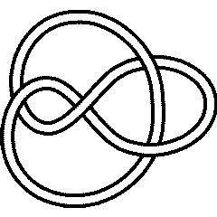 4_1 |
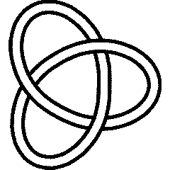 3_1 |
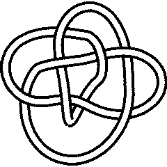 8_17 |
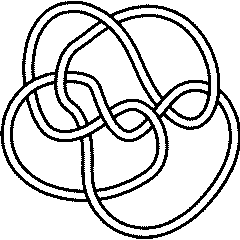 9_32 |
Unknotting Number
The unknotting number of a knot is the minimal number of crossing changes needed in order to unknot .
|
| ||||||||
Of the 512 knots whose unknotting number is known to KnotTheory`, 197 have unknotting number 1, 247 have unknotting number 2, 54 have unknotting number 3, 12 have unknotting number 4 and 1 has unknotting number 5:
In[11]:=
|
Plus @@ u /@ Cases[UnknottingNumber /@ AllKnots[], _Integer]
|
Out[11]=
|
u[0] + 197 u[1] + 247 u[2] + 54 u[3] + 12 u[4] + u[5]
|
There are 4 knots with up to 9 crossings whose unknotting number is unknown:
In[12]:=
|
Select[AllKnots[],
  Crossings[#] <= 9 && Head[UnknottingNumber[#]] === List &
]
|
Out[12]=
|
{Knot[9, 10], Knot[9, 13], Knot[9, 35], Knot[9, 38]}
|
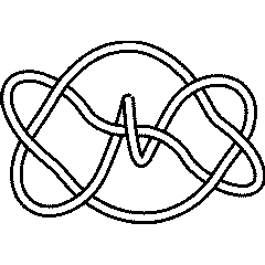 9_10 |
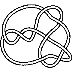 9_13 |
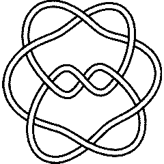 9_35 |
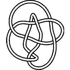 9_38 |
3-Genus
A Seifert surface for a knot is a compact oriented surface with boundary . Seifert surfaces exist, but are not unique. The SeifertView programme is a visual implementation of the algorithm of Seifert (1934) for the construction of a Seifert surface from a knot projection. The 3-genus of a knot is the minimal genus of a Seifert surface for that knot.
|
| ||||||||
The highest 3-genus of the knots known to KnotTheory` is , and there is only one knot with up to 11 crossings whose 3-genus is 5:
In[15]:=
|
Max[ThreeGenus /@ AllKnots[]]
|
Out[15]=
|
5
|
In[16]:=
|
Select[AllKnots[], ThreeGenus[#] == 5 &]
|
Out[16]=
|
{Knot[11, Alternating, 367]}
|
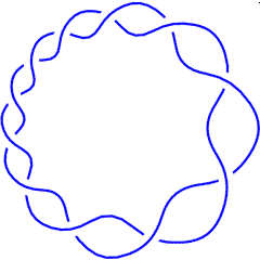 K11a367 |
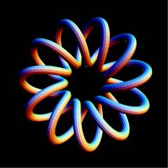 T(11,2) |
(K11a367 is, of couse, also known as the torus knot T(11,2)).
The Conway knot K11n34 is the closure of the braid BR[4, {1, 1, 2, -3, 2, 1, -3, -2, -2, -3, -3}]. Let us compute its 3-genus and compare it with the 3-genus of its mutant companion, the Kinoshita-Terasaka knot K11n42:
In[17]:=
|
ThreeGenus[BR[4, {1, 1, 2, -3, 2, 1, -3, -2, -2, -3, -3}]]
|
Out[17]=
|
3
|
In[18]:=
|
ThreeGenus[Knot[11, NonAlternating, 42]]
|
Out[18]=
|
2
|
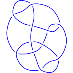 K11n34 |
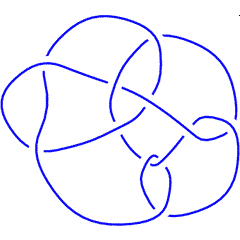 K11n42 |
Bridge Index
The bridge index' of a knot is the minimal number of local maxima (or local minima) in a generic smooth embedding of in .
|
| ||||||||
An often studied class of knots is the class of 2-bridge knots, knots whose bridge index is 2. Of the 49 prime 9-crossings knots, 24 are 2-bridge:
In[21]:=
|
Select[AllKnots[], Crossings[#] == 9 && BridgeIndex[#] == 2 &]
|
Out[21]=
|
{Knot[9, 1], Knot[9, 2], Knot[9, 3], Knot[9, 4], Knot[9, 5],

  Knot[9, 6], Knot[9, 7], Knot[9, 8], Knot[9, 9], Knot[9, 10],

  Knot[9, 11], Knot[9, 12], Knot[9, 13], Knot[9, 14], Knot[9, 15],

  Knot[9, 17], Knot[9, 18], Knot[9, 19], Knot[9, 20], Knot[9, 21],

  Knot[9, 23], Knot[9, 26], Knot[9, 27], Knot[9, 31]}
|
Super Bridge Index
The super bridge index of a knot is the minimal number, in a generic smooth embedding of in , of the maximal number of local maxima (or local minima) in a rigid rotation of that projection.
|
| ||||||||
Nakanishi Index
|
| ||||||||
Synthesis
In[26]:=
|
Profile[K_] := Profile[
  SymmetryType[K], UnknottingNumber[K], ThreeGenus[K],
  BridgeIndex[K], SuperBridgeIndex[K], NakanishiIndex[K]
]
|
In[27]:=
|
Profile[Knot[9,24]]
|
Out[27]=
|
Profile[Reversible, 1, 3, 3, {4, 6}, 1]
|
In[28]:=
|
Ks = Select[AllKnots[], (Crossings[#] == 9 && Profile[#]==Profile[Knot[9,24]])&]
|
Out[28]=
|
{Knot[9, 24], Knot[9, 28], Knot[9, 30], Knot[9, 34]}
|
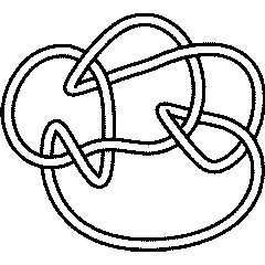 9_24 |
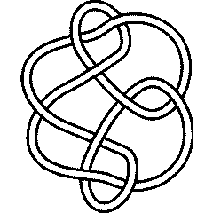 9_28 |
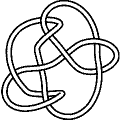 9_30 |
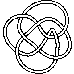 9_34 |
In[29]:=
|
Alexander[#][t]& /@ Ks
|
Out[29]=
|
       -3   5    10             2    3
{13 - t   + -- - -- - 10 t + 5 t  - t ,
             2   t
            t

         -3   5    12             2    3
  -15 + t   - -- + -- + 12 t - 5 t  + t ,
               2   t
              t

        -3   5    12             2    3
  17 - t   + -- - -- - 12 t + 5 t  - t ,
              2   t
             t

        -3   6    16             2    3
  23 - t   + -- - -- - 16 t + 6 t  - t }
              2   t
             t
|


